PDF

Action on Structures Exposed to Fire
— Thermal Elongation
Introduction
This is the 4th verification example from (Ref. 1) which is part of the European Standard EN-1991-1-2:2010-12, Eurocode 1: Actions on structures - Part 1-2: General actions - Actions on structures exposed to fire. It verifies that the calculated elongation matches the expected values.
Model Definition
The modeled geometry is a cube with side length of 100 mm. The temperature in the block is homogeneous and prescribed. The thermal strain function dL (Figure 1) is given in (Ref. 2).
Figure 1: Temperature dependent thermal strain function.
The model is a pure structural mechanics problem. The thermal expansion is calculated according to
with the given thermal strain function dL, the reference temperature Tref = 20°C and the prescribed temperature T (Table 1).
Results and Discussion
The reference and calculated values are given in Table 1 and match exactly. This is expected, because the thermal strain function prescribes the deformation and the deformation is what you compute.
References
1. DIN EN 1991-1-2/NA, National Annex - Nationally determined parameters - Eurocode 1: Actions on structures - Part 1-2: General actions - Actions on structures exposed to fire
2. DIN EN 1993-1-2 Eurocode 3: Design of steel structures - Part 1-2: General rules - Structural fire design; German version EN 1993-1-2:2005 + AC:2009
Application Library path: Heat_Transfer_Module/Verification_Examples/fire_effects_thermal_elongation
Modeling Instructions
From the File menu, choose New.
New
In the New window, click  Model Wizard.
Model Wizard
1
In the Model Wizard window, click  3D.
2
In the Select Physics tree, select Structural Mechanics>Solid Mechanics (solid).
3
Click Add.
4
Click  Study.
5
In the Select Study tree, select General Studies>Stationary.
6
Geometry 1
Define a parameter for the temperature which is the input for the thermal expansion. A parametric sweep over this temperature will be performed.
Global Definitions
Parameters 1
1
In the Model Builder window, under Global Definitions click Parameters 1.
2
In the Settings window for Parameters, locate the Parameters section.
3
Geometry 1
1
In the Model Builder window, under Component 1 (comp1) click Geometry 1.
2
In the Settings window for Geometry, locate the Units section.
3
From the Length unit list, choose mm.
Block 1 (blk1)
1
In the Geometry toolbar, click  Block.
2
In the Settings window for Block, locate the Size and Shape section.
3
In the Width text field, type 100.
4
In the Depth text field, type 100.
5
In the Height text field, type 100.
6
Click  Build All Objects.
Materials
Define the material properties for steel.
Steel
1
In the Model Builder window, under Component 1 (comp1) right-click Materials and choose Blank Material.
2
In the Settings window for Material, type Steel in the Label text field.
3
Locate the Material Contents section. In the table, enter the following settings:
4
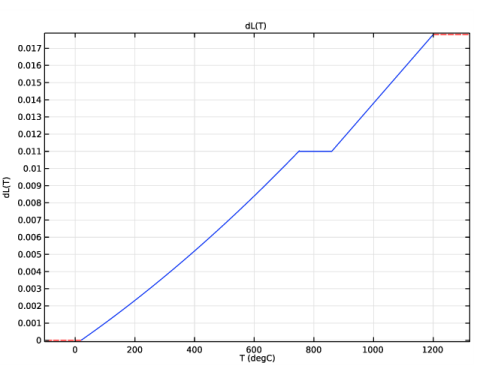
Locate the Material Properties section. In the Material properties tree, select Solid Mechanics>Thermal Expansion>Thermal strain (dL).
5
Click  Add to Material.
Piecewise 1 (pw1)
1
In the Model Builder window, expand the Component 1 (comp1)>Materials>Steel (mat1) node.
2
Right-click Component 1 (comp1)>Materials>Steel (mat1)>Thermal expansion (ThermalExpansion) and choose Functions>Piecewise.
3
In the Settings window for Piecewise, type dL in the Function name text field.
4
Locate the Definition section. In the Argument text field, type T.
5
Find the Intervals subsection. In the table, enter the following settings:
6
Locate the Units section. In the Arguments text field, type degC.
7
Click  Plot. Compare with Figure 1.
Steel (mat1)
1
In the Model Builder window, under Component 1 (comp1)>Materials>Steel (mat1) click Thermal expansion (ThermalExpansion).
2
In the Settings window for Thermal Expansion, locate the Output Properties section.
3
The variable T is not known, yet. Add the temperature in the Model Inputs section to define it.
4
Locate the Model Inputs section. Click  Select Quantity.
5
In the Physical Quantity dialog box, type temperature in the text field.
6
Click  Filter.
7
In the tree, select General>Temperature (K).
8
Solid Mechanics (solid)
Roller 1
1
In the Model Builder window, under Component 1 (comp1) right-click Solid Mechanics (solid) and choose Roller.
2
The roller condition ensures that the structure expands in all directions uniformly.
Linear Elastic Material 1
In the Model Builder window, click Linear Elastic Material 1.
Thermal Expansion 1
1
In the Physics toolbar, click  Attributes and choose Thermal Expansion.
2
In the Settings window for Thermal Expansion, locate the Thermal Expansion Properties section.
3
From the Input type list, choose Thermal strain.
Define a parameter for the input temperature.
4
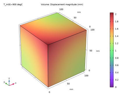
Locate the Model Input section. From the T list, choose User defined. In the associated text field, type T_in.
Mesh 1
Swept 1
In the Mesh toolbar, click  Swept.
Size
1
In the Model Builder window, click Size.
2
In the Settings window for Size, locate the Element Size section.
3
From the Predefined list, choose Extremely coarse.
4
Click  Build All.
A very coarse mesh is sufficient. Even just one element would be enough, because the deformation is prescribed and you verify that the calculated deformation gives the same value. This is a basic test to validate that the tested functionality works correctly.
Study 1
Step 1: Stationary
Set up a parametric sweep over the input temperature.
Parametric Sweep
1
In the Study toolbar, click  Parametric Sweep.
2
In the Settings window for Parametric Sweep, locate the Study Settings section.
3
4
5
In the Study toolbar, click  Compute.
A 3D stress plot is created automatically. Add a new plot group to visualize the displacement field.
Results
Displacement field
1
In the Home toolbar, click  Add Plot Group and choose 3D Plot Group.
2
In the Settings window for 3D Plot Group, type Displacement field in the Label text field.
Volume 1
1
Right-click Displacement field and choose Volume.
2
In the Settings window for Volume, locate the Coloring and Style section.
3
Click  Change Color Table.
4
In the Color Table dialog box, select Rainbow>SpectrumLight in the tree.
5
6
In the Displacement field toolbar, click  Plot.
Surface Average 1
1
In the Results toolbar, click  More Derived Values and choose Average>Surface Average.
2
3
In the Settings window for Surface Average, locate the Expressions section.
4
5
Click  Evaluate.
Table
1
Go to the Table window.
To compare these results with the reference values, import the data as interpolation function.
Global Definitions
Interpolation 1 (int1)
1
In the Home toolbar, click  Functions and choose Global>Interpolation.
2
In the Settings window for Interpolation, locate the Definition section.
3
From the Data source list, choose File.
4
Click  Browse.
5
6
Find the Functions subsection. In the table, enter the following settings:
7
Locate the Units section. In the Argument table, enter the following settings:
8
Locate the Definition section. Click  Import.
It is not necessary to compute the whole study again. To make the data available for postprocessing, just update the solution.
Study 1
In the Study toolbar, click  Update Solution.
Results
Surface Average 1
1
In the Model Builder window, under Results>Derived Values click Surface Average 1.
2
In the Settings window for Surface Average, locate the Expressions section.
3
4
In the Results toolbar, click  Evaluate and choose Clear and Evaluate All.
Table
1
Go to the Table window.
The computed and reference values match exactly. Compare with Table 1.