|
|
|

|
1
|
|
2
|
|
3
|
Click Add.
|
|
4
|
Click
|
|
5
|
|
6
|
Click
|
|
1
|
|
2
|
|
1
|
|
2
|
|
3
|
|
1
|
|
2
|
|
3
|
|
4
|
|
5
|
|
6
|
|
1
|
|
2
|
|
3
|
|
4
|
|
5
|
|
6
|
|
7
|
|
1
|
|
2
|
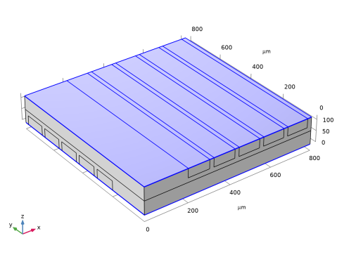
Select the object blk2 only.
|
|
3
|
|
4
|
|
5
|
|
6
|
|
7
|
Locate the Selections of Resulting Entities section. Find the Cumulative selection subsection. Click New.
|
|
8
|
|
9
|
Click OK.
|
|
1
|
|
2
|
Click in the Graphics window and then press Ctrl+A to select all objects.
|
|
3
|
|
4
|
|
5
|
|
6
|
|
7
|
|
8
|
|
9
|
|
10
|
|
11
|
|
12
|
|
1
|
|
2
|
|
3
|
|
1
|
|
2
|
|
3
|
|
1
|
|
2
|
|
3
|
|
1
|
|
2
|
|
3
|
|
1
|
|
2
|
|
3
|
|
4
|
|
1
|
|
2
|
|
3
|
|
4
|
|
5
|
|
6
|
Click OK.
|
|
1
|
|
2
|
|
3
|
|
1
|
|
2
|
|
3
|
|
4
|
|
5
|
|
1
|
|
2
|
|
1
|
In the Model Builder window, under Component 1 (comp1) click Heat Transfer in Solids and Fluids (ht).
|
|
2
|
|
3
|
|
1
|
In the Model Builder window, under Component 1 (comp1)>Heat Transfer in Solids and Fluids (ht) click Fluid 1.
|
|
2
|
|
3
|
|
1
|
|
2
|
|
3
|
|
4
|
|
1
|
|
2
|
|
3
|
|
4
|
|
1
|
|
2
|
|
3
|
|
1
|
|
2
|
|
3
|
|
1
|
|
2
|
|
3
|
|
1
|
|
2
|
|
3
|
|
4
|
|
1
|
|
2
|
|
3
|
|
4
|
|
5
|
|
1
|
|
2
|
|
3
|
|
4
|
|
5
|
|
1
|
|
2
|
|
3
|
|
1
|
|
2
|
|
3
|
|
1
|
|
2
|
|
3
|
|
1
|
In the Model Builder window, under Component 1 (comp1)>Multiphysics click Nonisothermal Flow 1 (nitf1).
|
|
2
|
|
3
|
|
1
|
|
2
|
|
3
|
|
1
|
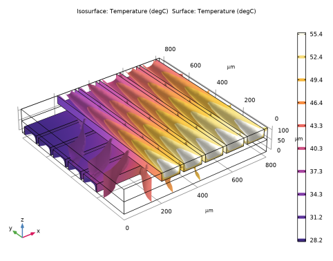
In the Model Builder window, expand the Results>Isothermal Contours (ht) node, then click Isosurface.
|
|
2
|
|
3
|
|
1
|
|
2
|
|
3
|
|
4
|
|
5
|
Click Replace Expression in the upper-right corner of the Expression section. From the menu, choose Component 1 (comp1)>Heat Transfer in Solids and Fluids>Temperature>T - Temperature - K.
|
|
6
|
|
7
|
|
1
|
|
2
|
|
1
|
|
2
|
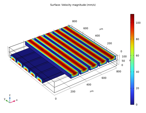
In the Settings window for Surface, click Replace Expression in the upper-right corner of the Expression section. From the menu, choose Component 1 (comp1)>Laminar Flow>Velocity and pressure>spf.U - Velocity magnitude - m/s.
|
|
3
|
|
4
|
|
1
|
|
2
|
|
3
|
|
1
|
|
2
|
|
1
|
|
2
|
|
3
|
|
4
|
|
5
|
|
6
|
|
7
|
Click OK.
|
|
8
|
|
1
|
|
2
|
|
3
|
Click Replace Expression in the upper-right corner of the Expressions section. From the menu, choose Component 1 (comp1)>Heat Transfer in Solids and Fluids>Temperature>Weighted average temperature>ht.ofl1.Tave - Weighted average temperature - K.
|
|
4
|
Locate the Expressions section. In the table, enter the following settings:
|
|
5
|
Click
|
|
1
|
Go to the Table window.
|
|
1
|
|
2
|
|
3
|
|
4
|
Click Replace Expression in the upper-right corner of the Expressions section. From the menu, choose Component 1 (comp1)>Laminar Flow>Velocity and pressure>p - Pressure - Pa.
|
|
5
|
|
6
|
Locate the Expressions section. In the table, enter the following settings:
|
|
7
|
Click
|
|
1
|
Go to the Table window.
|
|
1
|
|
2
|
|
4
|
|
5
|
Click
|
|
1
|
Go to the Table window.
|