You are viewing the documentation for an older COMSOL version. The latest version is available here.
PDF

Temperature Field in a Cooling Flange
Introduction
Chemical reaction fluids can be cooled using glass flanges. The reaction fluid is passed through the flange and the air surrounding the flange then serves as the coolant. Engineers looking to optimize the cooling performance of such flanges can look to simulation for help.
Figure 1: Operating principle of the cooling flange.
First off, the physics to analyze in this case is heat transfer, involving both convection and conduction. Heat transfer occurs via convection with both interior and exterior surfaces of the flange, and via conduction through the glass. The tube is heated from the inside by the process fluid, conduction then diffuses the heat in the flange, which in turn heats the air, causing a convective flow due to buoyancy effects. The cooling performance of the flange therefore depends on both convection and conduction.
To simplify the simulation convection cooling is analyzed using the heat transfer coefficient, h. Since this describes the fluid flow influence and the convective fluxes, the flow field does not have to be computed.
This particular example uses external research data (Ref. 1) for the outer surface heat transfer coefficient, which was originally obtained through semi-empirical data for natural convection around a cylinder. For the tube-facing surface a coefficient for forced convection in a tube is used.
Model Definition
Figure 2 presents the modeled geometry.
Figure 2: Drawing of the cooling flange.
The glass flange consists of a 4 mm thick pipe and 4 mm thick and 10 mm tall flanges, with a connecting pipe that has a 3 mm thick wall and an inner diameter of 16 mm. Note that in this tutorial, a parametric study on the pipe inner diameter is performed while the other dimensions remain fixed.
During operation, the hot process fluid heats the inside of the tube. The flange conducts the heat and transfers it to the surrounding air. As the air is heated, buoyancy effects cause a convective flow.
The heat transfer within the flange is described by the stationary heat equation
where k is the thermal conductivity (W/(m·K)), and T is the temperature (K). On the flange’s exterior boundaries, which face the air and process fluid, the applicable boundary condition is
where n is the normal vector of the boundary, h, is the heat transfer coefficient (W/(m2·K)), and Tinf is the temperature of the surrounding medium (K). For this simulation, set Text to 298 K for the cooling air and to 363 K for the process fluid.
You can approximate the value for the heat transfer coefficient, h, on the process fluid side with a constant value of 15 W/(m2·K) because the fluid’s velocity is close to constant and the model assumes that its temperature decreases only slightly.
The h expression on the air side is more elaborate. Assume that the free-convection process around the flange is similar to that around a cylinder. The heat transfer coefficient for a cylinder is available in the literature (Ref. 1), and you can use the expression
where k is the thermal conductivity of air (26.2 mW/(m·K) at 298 K); L is the typical length, which in this case is the outer diameter of the flange (44 mm); and f(θ) is an empirical coefficient tabulated in Table 1 as a function of the incidence angle θ, which is shown in Figure 3. Finally, Gr is the Grashof number defined as
where αp is the coefficient of thermal expansion (1/K), which equals that for an ideal gas, g is the gravitational acceleration (9.81 m/s2), and ν is the kinematic viscosity
(18·106 m2/s). For the flange material, use silica glass.
θ (deg)
f(θ)
Figure 3: Definition of the incidence angle θ.
Results and Discussion
Figure 4 shows the flange surface temperature at steady state.
Figure 4: Stationary surface temperature of the flange.
As you can see in the surface temperature plot above to the left, the tube surface temperature is about 13 K higher than the flange shoulders. From the results, we can learn that the heat transfer from the outer surfaces of the flange is pretty efficient; there is a temperature difference of roughly 19 K between the outer flange surface and the air stream.
Figure 5 shows the heat transfer coefficient for the flange’s outer walls.
Figure 5: Heat transfer film coefficient, h, for the flange’s outer walls.
As you can see, the coefficient decreases significantly along the vertical position of the flange’s outer boundary.
Calculating the flange’s total cooling power by integrating the normal total heat flux over the outer surfaces gives a value of 0.51 W which correspond to 1.02 W for the full geometry.
The surface temperature plot shown on Figure 4 further gives light to an inefficiency in the current flange design. When it enters the flange the process fluid is 363 K, while the inner surface of the pipe is only 32 K lower. Increasing the tube diameter would improve the heat transfer here, which is performed in a second stage of the modeling by varying the pipe’s diameter, but keeping all other factors constant. By plotting in Figure 6 the global cooling power as a function of the inner pipe radius, you can now analyze how altering the radius impacts the performance of the cooling flange.
Figure 6: Total cooling power versus inner pipe radius.
Reference
1. B. Sundén, Kompendium i värmeöverföring [Notes on Heat Transfer], Sec. 10-3, Dept. of Heat and Power Engineering, Lund Inst. of Technology, 2003 (in Swedish).
Application Library path: Heat_Transfer_Module/Thermal_Processing/cooling_flange
Modeling Instructions
From the File menu, choose New.
New
In the New window, click  Model Wizard.
Model Wizard
1
In the Model Wizard window, click  3D.
2
In the Select Physics tree, select Heat Transfer>Heat Transfer in Solids (ht).
3
Click Add.
4
Click  Study.
5
In the Select Study tree, select General Studies>Stationary.
6
Global Definitions
Parameters 1
Define parameters for relevant temperatures, material properties, and geometric dimensions. The parameters related to the geometry dimensions make it easier to perform parametric studies where you let some of these dimensions vary.
1
In the Model Builder window, under Global Definitions click Parameters 1.
2
In the Settings window for Parameters, locate the Parameters section.
3
Next, create an interpolation function defined by the data in Table 1.
Interpolation 1 (int1)
1
In the Home toolbar, click  Functions and choose Global>Interpolation.
2
In the Settings window for Interpolation, locate the Definition section.
3
In the Function name text field, type f.
4
5
Locate the Units section. In the Argument table, enter the following settings:
6
In the Function table, enter the following settings:
7
Geometry 1
In a first geometry modeling stage, create a 2D geometry by following the steps below.
Work Plane 1 (wp1)
1
In the Geometry toolbar, click  Work Plane.
2
In the Settings window for Work Plane, click  Show Work Plane.
Work Plane 1 (wp1)>Plane Geometry
In the Model Builder window, click Plane Geometry.
Work Plane 1 (wp1)>Rectangle 1 (r1)
1
In the Work Plane toolbar, click  Rectangle.
2
In the Settings window for Rectangle, locate the Size and Shape section.
3
In the Width text field, type 2*wf.
4
In the Height text field, type t2.
5
Locate the Position section. In the yw text field, type r_inner.
6
In the Work Plane toolbar, click  Build All.
7
Click the  Zoom Extents button in the Graphics toolbar.
Work Plane 1 (wp1)>Quadratic Bézier 1 (qb1)
1
In the Work Plane toolbar, click  More Primitives and choose Quadratic Bézier.
2
In the Settings window for Quadratic Bézier, locate the Control Points section.
3
In row 1, set yw to r_inner+t2.
4
In row 2, set xw to wf/2, and yw to r_inner+t2.
5
In row 3, set xw to wf/2, and yw to r_inner+t2+wf/2.
Work Plane 1 (wp1)>Line Segment 1 (ls1)
1
In the Work Plane toolbar, click  More Primitives and choose Line Segment.
2
In the Settings window for Line Segment, locate the Starting Point section.
3
From the Specify list, choose Coordinates.
4
Locate the Endpoint section. From the Specify list, choose Coordinates.
5
Locate the Starting Point section. In the xw text field, type wf/2.
6
Locate the Endpoint section. In the xw text field, type 3*wf/2.
7
Locate the Starting Point section. In the yw text field, type r_inner+t2+wf/2.
8
Locate the Endpoint section. In the yw text field, type r_inner+t2+wf/2.
Work Plane 1 (wp1)>Quadratic Bézier 2 (qb2)
1
In the Work Plane toolbar, click  More Primitives and choose Quadratic Bézier.
2
In the Settings window for Quadratic Bézier, locate the Control Points section.
3
In row 1, set xw to 3*wf/2, and yw to r_inner+t2+wf/2.
4
In row 2, set xw to 3*wf/2, and yw to r_inner+t2.
5
In row 3, set xw to 2*wf, and yw to r_inner+t2.
Work Plane 1 (wp1)>Line Segment 2 (ls2)
1
In the Work Plane toolbar, click  More Primitives and choose Line Segment.
2
In the Settings window for Line Segment, locate the Starting Point section.
3
From the Specify list, choose Coordinates.
4
Locate the Endpoint section. From the Specify list, choose Coordinates.
5
Locate the Starting Point section. In the yw text field, type r_inner+t2.
6
Locate the Endpoint section. In the xw text field, type 2*wf.
7
In the yw text field, type r_inner+t2.
8
Drag and drop below Quadratic Bézier 2 (qb2).
Work Plane 1 (wp1)>Convert to Solid 1 (csol1)
1
In the Work Plane toolbar, click  Conversions and choose Convert to Solid.
2
Select the objects ls1, ls2, qb1, and qb2 only.
3
In the Work Plane toolbar, click  Build All.
4
Click the  Zoom Extents button in the Graphics toolbar.
Work Plane 1 (wp1)>Rectangle 2 (r2)
1
In the Work Plane toolbar, click  Rectangle.
2
In the Settings window for Rectangle, locate the Size and Shape section.
3
In the Width text field, type wf.
4
In the Height text field, type hf-wf.
5
Locate the Position section. In the xw text field, type wf/2.
6
In the yw text field, type r_inner+t2+wf/2.
7
In the Work Plane toolbar, click  Build All.
8
Click the  Zoom Extents button in the Graphics toolbar.
Work Plane 1 (wp1)>Circle 1 (c1)
1
In the Work Plane toolbar, click  Circle.
2
In the Settings window for Circle, locate the Size and Shape section.
3
In the Radius text field, type wf/2.
4
In the Sector angle text field, type 180.
5
Locate the Position section. In the xw text field, type wf.
6
In the yw text field, type r_inner+t2+hf-wf/2.
7
In the Work Plane toolbar, click  Build All.
8
Click the  Zoom Extents button in the Graphics toolbar.
Work Plane 1 (wp1)>Array 1 (arr1)
1
In the Work Plane toolbar, click  Transforms and choose Array.
2
Click in the Graphics window and then press Ctrl+A to select all objects.
3
In the Settings window for Array, locate the Size section.
4
From the Array type list, choose Linear.
5
In the Size text field, type 3.
6
Locate the Displacement section. In the xw text field, type 2*wf.
7
In the Work Plane toolbar, click  Build All.
8
Click the  Zoom Extents button in the Graphics toolbar.
Work Plane 1 (wp1)>Polygon 1 (pol1)
1
In the Work Plane toolbar, click  Polygon.
2
In the Settings window for Polygon, locate the Object Type section.
3
From the Type list, choose Open curve.
4
Locate the Coordinates section. From the Data source list, choose Vectors.
5
In the xw text field, type 0 0 -l1 -l1 -l1 -l1 -2*l1/3.
6
In the yw text field, type r_inner+t2 r_inner r_inner r_inner r_inner+t1 r_inner+t1 r_inner+t1.
Work Plane 1 (wp1)>Cubic Bézier 1 (cb1)
1
In the Work Plane toolbar, click  More Primitives and choose Cubic Bézier.
2
In the Settings window for Cubic Bézier, locate the Control Points section.
3
In row 1, set xw to -2*l1/3, and yw to r_inner+t2.
4
In row 2, set xw to -l1/3, and yw to r_inner+t2.
5
In row 3, set xw to -l1/3, and yw to r_inner+t2.
6
In row 4, set yw to r_inner+t2.
Work Plane 1 (wp1)>Convert to Solid 2 (csol2)
1
In the Work Plane toolbar, click  Conversions and choose Convert to Solid.
2
Select the objects cb1 and pol1 only.
3
In the Work Plane toolbar, click  Build All.
4
Click the  Zoom Extents button in the Graphics toolbar.
5
In the Model Builder window, right-click Geometry 1 and choose Build All.
You obtain the following 2D geometry.
Next, revolve the embedded 2D geometry to create the 3D model geometry.
Revolve 1 (rev1)
1
In the Geometry toolbar, click  Revolve.
2
In the Settings window for Revolve, locate the Revolution Angles section.
3
Click the Angles button.
4
In the End angle text field, type 180.
5
Locate the Revolution Axis section. Find the Direction of revolution axis subsection. In the xw text field, type 1.
6
In the yw text field, type 0.
7
In the Geometry toolbar, click  Build All.
8
Click the  Go to Default View button in the Graphics toolbar.
Definitions
Variables 1
1
In the Home toolbar, click  Variables and choose Local Variables.
2
In the Settings window for Variables, locate the Geometric Entity Selection section.
3
From the Geometric entity level list, choose Boundary.
4
To do this, first copy the list of boundaries from this text, then use the Paste Selection button in the Geometric Entity Selection section, to paste these numbers.
For use when specifying the boundary condition for the flange’s outer surface, create a selection.
5
Click  Create Selection.
6
In the Create Selection dialog box, type Outer Boundaries in the Selection name text field.
7
8
In the Settings window for Variables, locate the Variables section.
9
Add Material
1
In the Home toolbar, click  Add Material to open the Add Material window.
2
Go to the Add Material window.
3
In the tree, select Built-in>Silica glass.
4
Click Add to Component in the window toolbar.
5
In the Home toolbar, click  Add Material to close the Add Material window.
Definitions
Ambient Properties 1 (ampr1)
1
In the Physics toolbar, click  Shared Properties and choose Ambient Properties.
2
In the Settings window for Ambient Properties, locate the Ambient Conditions section.
3
In the Tamb text field, type 298[K].
Heat Transfer in Solids (ht)
The next steps set the temperature shape function to Quadratic serendipity in order to reduce computational costs without significant deterioration in accuracy.
1
In the Model Builder window, under Component 1 (comp1) click Heat Transfer in Solids (ht).
2
In the Settings window for Heat Transfer in Solids, click to expand the Discretization section.
3
From the Temperature list, choose Quadratic serendipity.
Initial Values 1
1
In the Model Builder window, under Component 1 (comp1)>Heat Transfer in Solids (ht) click Initial Values 1.
2
In the Settings window for Initial Values, locate the Initial Values section.
3
In the T text field, type 323.15[K].
Symmetry 1
1
In the Physics toolbar, click  Boundaries and choose Symmetry.
2
Click the  Wireframe Rendering button in the Graphics toolbar.
3
Heat Flux 1
1
In the Physics toolbar, click  Boundaries and choose Heat Flux.
2
3
In the Settings window for Heat Flux, locate the Heat Flux section.
4
From the Flux type list, choose Convective heat flux.
5
In the h text field, type Hh.
6
In the Text text field, type T_inner.
7
Click the  Wireframe Rendering button in the Graphics toolbar to go back to the original view.
Heat Flux 2
1
In the Physics toolbar, click  Boundaries and choose Heat Flux.
2
In the Settings window for Heat Flux, locate the Boundary Selection section.
3
From the Selection list, choose Outer Boundaries.
4
Locate the Heat Flux section. From the Flux type list, choose Convective heat flux.
5
In the h text field, type Hc.
6
From the Text list, choose Ambient temperature (ampr1).
Mesh 1
Mapped 1
1
In the Mesh toolbar, click  Boundary and choose Mapped.
2
Click the  Go to XY View button in the Graphics toolbar. Do this twice to see the boundary mesh.
3
Size 1
1
In the Mesh toolbar, click Size Attribute and choose Extra Fine.
2
In the Settings window for Size, click  Build Selected.
Free Triangular 1
1
In the Mesh toolbar, click  Boundary and choose Free Triangular.
2
3
In the Settings window for Free Triangular, click  Build Selected.
4
Click the  Go to Default View button in the Graphics toolbar.
Swept 1
In the Mesh toolbar, click  Swept.
Distribution 1
1
Right-click Swept 1 and choose Distribution.
2
In the Settings window for Distribution, locate the Distribution section.
3
In the Number of elements text field, type 30.
4
Click  Build All.
Study 1
In the Home toolbar, click  Compute.
Results
Temperature (ht)
The first default plot group shows the temperature field on the surface. To get a more intuitive view with gravity along the vertical, rotate the geometry in the Graphics window. You can preserve a view for a plot by creating a View feature node as follows:
1
Click the  Show More Options button in the Model Builder toolbar.
2
In the Show More Options dialog box, in the tree, select the check box for the node Results>Views.
3
View 3D 3
1
In the Model Builder window, under Results right-click Views and choose View 3D.
2
Use the Graphics toolbox to get a satisfying view.
3
In the Settings window for View 3D, locate the View section.
4
Select the Lock camera check box.
Next, apply the view to the temperature plot.
Temperature (ht)
1
In the Model Builder window, under Results click Temperature (ht).
2
In the Settings window for 3D Plot Group, locate the Plot Settings section.
3
From the View list, choose View 3D 3.
4
In the Temperature (ht) toolbar, click  Plot.
Compare with Figure 4.
Delete the second plot group to make a new surface plot of the heat transfer film coefficient.
Isothermal Contours (ht)
1
In the Model Builder window, under Results right-click Isothermal Contours (ht) and choose Delete.
2
Click Yes to confirm.
Heat Transfer Film Coefficient
1
In the Home toolbar, click  Add Plot Group and choose 3D Plot Group.
2
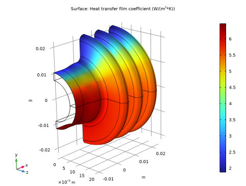
In the Settings window for 3D Plot Group, type Heat Transfer Film Coefficient in the Label text field.
3
Locate the Plot Settings section. From the View list, choose View 3D 3.
Surface 1
1
In the Heat Transfer Film Coefficient toolbar, click  Surface.
2
In the Settings window for Surface, click Replace Expression in the upper-right corner of the Expression section. From the menu, choose Component 1 (comp1)>Definitions>Variables>Hc - Heat transfer film coefficient - W/(m²·K).
3
In the Heat Transfer Film Coefficient toolbar, click  Plot.
Compare this plot with that in Figure 5.
Outgoing Heat Flux
1
In the Results toolbar, click  More Derived Values and choose Integration>Surface Integration.
2
In the Settings window for Surface Integration, type Outgoing Heat Flux in the Label text field.
3
Locate the Selection section. From the Selection list, choose Outer Boundaries.
4
Click Replace Expression in the upper-right corner of the Expressions section. From the menu, choose Component 1 (comp1)>Heat Transfer in Solids>Boundary fluxes>ht.ntflux - Normal total heat flux - W/m².
5
Click  Evaluate.
Table
1
Go to the Table window.
The integrated value, approximately 0.51 W, appears in the Table tab below the Graphics window. Taking both flange halves into account, the total cooling power of the flange is thus roughly 1 W.
Finally, extend the model by performing a parametric sweep over the inner pipe radius. Before adding a separate study for this purpose, define a variable for the total cooling power.
Definitions
Integration, Outer
1
In the Definitions toolbar, click  Nonlocal Couplings and choose Integration.
2
In the Settings window for Integration, type Integration, Outer in the Label text field.
3
In the Operator name text field, type intop_outer.
4
Locate the Source Selection section. From the Geometric entity level list, choose Boundary.
5
From the Selection list, choose Outer Boundaries.
Variables 2
1
In the Definitions toolbar, click  Local Variables.
2
In the Settings window for Variables, locate the Variables section.
3
Add Study
1
In the Home toolbar, click  Add Study to open the Add Study window.
2
Go to the Add Study window.
3
Find the Studies subsection. In the Select Study tree, select General Studies>Stationary.
4
Click Add Study in the window toolbar.
5
In the Home toolbar, click  Add Study to close the Add Study window.
Study 2
Parametric Sweep
1
In the Study toolbar, click  Parametric Sweep.
2
In the Settings window for Parametric Sweep, locate the Study Settings section.
3
4
This gives a sweep centered around the original radius value.
5
In the Study toolbar, click  Compute.
Results
Temperature (ht) 1
You get a new surface plot of the temperature for the parametric solution. From the Parameter value list, you can choose the radius value for which to display the result.
1
In the Settings window for 3D Plot Group, locate the Plot Settings section.
2
From the View list, choose View 3D 3.
Surface temperature for an inner radius of 10 mm.
Finally, replace the slice plot in the fourth plot group by a graph of the total cooling power versus tube radius.
Isothermal Contours (ht)
1
Right-click Isothermal Contours (ht) and choose Delete.
2
Click Yes to confirm.
Cooling Power
1
In the Home toolbar, click  Add Plot Group and choose 1D Plot Group.
2
In the Settings window for 1D Plot Group, type Cooling Power in the Label text field.
3
Locate the Data section. From the Dataset list, choose Study 2/Parametric Solutions 1 (sol3).
Global 1
1
In the Cooling Power toolbar, click  Global.
2
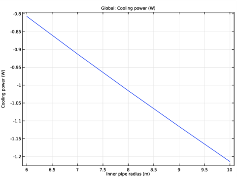
In the Settings window for Global, click Add Expression in the upper-right corner of the y-Axis Data section. From the menu, choose Component 1 (comp1)>Definitions>Variables>P_cooling - Cooling power - W.
3
Click to expand the Legends section. Clear the Show legends check box.
Cooling Power
1
In the Model Builder window, click Cooling Power.
2
In the Settings window for 1D Plot Group, locate the Plot Settings section.
3
Select the x-axis label check box. In the associated text field, type Inner pipe radius (m).
4
In the Cooling Power toolbar, click  Plot.
Compare the result with the graph in Figure 6.