PDF

Strength Reduction Method for Slope Stability
Introduction
The strength reduction method in combination with finite element analysis is a tool to find the factor of safety (FOS) in geomechanics, particularly for the stability of slopes and embankments. In the strength reduction method, the characteristic material properties are gradually reduced until failure occurs. Although the definition of an FOS depends on the context, in geotechnical problems it is defined with respect to the strength parameters of the soil, as discussed in Ref. 1.
The strength reduction method is applicable to linear failure criteria, like the Mohr–Coulomb criterion. When the Mohr–Coulomb criterion is used with the strength reduction method, the cohesion, the angle of internal friction, and the dilatation angle are simultaneously reduced until mechanical equilibrium is lost. Decreasing the material parameters results in a reduction of the shear strength of the soil, which eventually becomes unstable. This phenomena produces a collapse of the slope for a certain combination of loads, material parameters, and boundary conditions. The ratio between the initial cohesion and the cohesion at failure gives the FOS. More details of the method are given in Ref. 1 and Ref. 2.
The geometry, boundary conditions, loading conditions, and material parameters in this example are the same as discussed in Ref. 1. Quartic order shape functions are used to match the discretization used in Ref. 1. A similar example model can be found in Slope Stability in an Embankment Dam.
Model Definition
Figure 1 shows a cross section of the soil embankment. The lengths L1 and L2 are 85 m, and 20 m, respectively, and the heights of the embankment H1 and H2 are 20 m and 10 m, respectively. The slope angle α varies from 15° to 45°.
Figure 1: Geometry of the cross-section of an embankment.
The material properties for both associative and nonassociative plasticity are summarized in Table 1, and taken from Ref. 1
ν
ψ
ρ
A plane strain approximation is used to model the soil embankment in 2D. The effect of gravity is included. The material properties for the Mohr–Coulomb model are parameterized with respect to a factor of safety parameter, FOS. A parametric study increases the FOS parameter, thereby reducing the strength of the soil with every parameter step. The actual factor of safety is the value of the FOS parameter at which the model no longer converges, which is an indication of the collapse of the slope.
The Mohr–Coulomb yield function F and plastic potential Q are
(1)
(2)
where I1 is the first stress invariant and J2 is the second deviatoric stress invariant. The parameterized cohesion C, parameterized angle of internal friction Φ, and parameterized dilatation angle Φ are given in terms of the FOS,
(3)
where c is the cohesion, is the angle of internal friction, and ψ is the dilatation angle. Note that c, , and ψ are initial, unreduced material parameters. For the associative flow rule, .
For the nonassociative flow rule, ψ is kept constant as long as it is smaller than Φ, see Ref. 2 for details. However, in this example, ψ is zero when using the nonassociative flow rule, so no special treatment is needed, and Equation 3 is applicable to the associative as well as the nonassociative flow rule.
For the nonassociative flow rule, the strength reduction method might trigger numerical instabilities, which in turn can result in a nonunique failure surface and corresponding FOS. To avoid potential instabilities and convergence issues, the Davis procedure B approach, as suggested in Ref. 1 and Ref. 2, is used. In this approach, the associative flow rule is applied with reduced values of the cohesion and the angle of internal friction to capture the effects of the nonassociative flow rule. The reduced cohesion c' and the reduced angle of internal friction are given by
(4)
where the reduction factor β is
Hence, Equation 3 is rewritten in terms of the reduced cohesion c' and the reduced angle of internal friction for the associative and nonassociative flow rules, as the reduction factor β is unity for the associative flow rule.
Results and Discussion
The factor of safety (FOS) for different slope angles is shown in Figure 2. The FOS decreases as the slope angle increases, which is expected. The FOS for the same slope inclination with the nonassociative flow rule (material set 1) is always smaller than for the associative flow rule (material set 2), but the influence of the nonassociative flow rule is marginal for the material parameters chosen. The results presented in Figure 2 are in good agreement with the results presented in Figure 4 of Ref. 1.
Figure 2: Factor of safety versus slope angle.
The equivalent plastic strain for different slope angles just before collapse is shown in Figure 3 and Figure 4 for the two material sets. The localization of plastic strains in the figures gives an indication of the failure surface for different slope angles. It is evident that for lower slope angles, multiple failure surfaces develop in the embankment.
A 3D visualization of the displacement for a slope angle equal to 45° is shown in Figure 5 and Figure 6 for material sets 1 and 2, respectively. The results are qualitatively in good agreement with the results presented in Figure 2 of Ref. 1. The figures also clearly show how parts of the embankment outside the slip surface start sliding once the material becomes unstable.
Figure 3: Equivalent plastic strain just before collapse for material set 1 (nonassociative flow).
Figure 4: Equivalent plastic strain just before collapse for material set 2 (associative flow).
Figure 5: Displacement magnitude in the soil embankment just before slope collapse for material set 1 (nonassociative flow).
Figure 6: Displacement magnitude in the soil embankment just before slope collapse for material set 2 (associative flow).
Notes About the COMSOL Implementation
A Mesh Control Domain is added to the Geometry node in order to assign a denser mesh in the region where soil slippage is expected. The mesh control domain is removed from the geometry sequence once the mesh is generated, so this virtual domain is not visible in the physics selections.
Two stationary study steps are added. The first study step computes the in-situ stresses due to gravity. The Mohr–Coulomb criterion is added in the second study to compute the elastoplastic failure due to the combined effect of gravity and the reduction in strength, where the initial stresses generated in the first step are incorporated in the analysis with the help of an Initial Stress and Strain node.
Two outer parametric sweeps are added to change the slope angle and the set of material parameters.
Because the model stores a NaN solution corresponding to the nonconverged values of the FOS, the generation of default plots can be problematic, as default plots are set to portrait the last parameter value. Also, finding the last converged FOS parameter value manually for each value of the slope angle and material parameter set can be cumbersome. To avoid these issues, use a model method to generate a 1D plot for the factor of safety versus slope angle for each material parameter set. The model method also generates a von Mises stress plot, a 3D displacement plot, as well as plastic strain plots for each slope angle for the two material sets.
The model method is written assuming that a certain dataset tag is available and that the intended plots, functions, and datasets are not already created. Although fail-safe usage conditions and error messages are added, the model method could fail if the default material, geometry, study, or result parameters or nodes change. The model method then has to be modified according to the current model setup.
References
1. H.F.Schweiger “Strength reduction technique with finite element method for slopes without stabilization measures,” Benchmark, International Magazine for Engineers, Designers and Analysts from NAFEMS, pp. 51–58, 2020.
2. S. Oberhollenzer, F. Tschuchnigg, and H.F.Schweiger “Finite element analysis of slope stability problems using non-associated plasticity,” Journal of Rock Mechanics and Geotechnical Engineering, vol. 10, pp. 1091–1101, 2018.
Application Library path: Geomechanics_Module/Verification_Examples/strength_reduction_method
Modeling Instructions
From the File menu, choose New.
New
In the New window, click  Model Wizard.
Model Wizard
1
In the Model Wizard window, click  2D.
2
In the Select Physics tree, select Structural Mechanics>Solid Mechanics (solid).
3
4
Click  Study.
5
In the Select Study tree, select General Studies>Stationary.
6
Parameters for the model geometry, material, and solver are available in the appended text files.
Global Definitions
Geometry and Solver Parameters
1
In the Model Builder window, under Global Definitions click Parameters 1.
2
In the Settings window for Parameters, type Geometry and Solver Parameters in the Label text field.
3
Locate the Parameters section. Click  Load from File.
4
Material Parameters
1
In the Home toolbar, click  Parameters and choose Add>Parameters.
2
In the Settings window for Parameters, type Material Parameters in the Label text field.
3
Locate the Parameters section. Click  Load from File.
4
5
In the Home toolbar, click  Parameter Case.
6
In the Settings window for Case, type Material Parameter Set 1 in the Label text field.
7
In the Home toolbar, click  Parameter Case.
8
In the Settings window for Case, type Material Parameter Set 2 in the Label text field.
9
Locate the Parameters section. Click  Load from File.
10
Definitions
Define the parameterized cohesion and angle of internal friction for the Mohr-Coulomb criterion.
Variables 1
1
In the Model Builder window, expand the Component 1 (comp1)>Definitions node.
2
Right-click Definitions and choose Variables.
3
In the Settings window for Variables, locate the Variables section.
4
Geometry 1
Polygon 1 (pol1)
1
In the Geometry toolbar, click  Polygon.
2
In the Settings window for Polygon, locate the Coordinates section.
3
From the Data source list, choose Vectors.
4
In the x text field, type 0, L1,L1,L2+H2/tan(alpha),L2,0.
5
In the y text field, type 0, 0, H1+H2,H1+H2,H1,H1.
6
Click  Build Selected.
Polygon 2 (pol2)
In the Geometry toolbar, click  Polygon.
Split the geometry with a polygon to add a Mesh Control Domain.
1
In the Settings window for Polygon, locate the Object Type section.
2
From the Type list, choose Open curve.
3
Locate the Coordinates section. From the Data source list, choose Vectors.
4
In the x text field, type 0.8*L2,0.8*L2,1.3*L2+H2/tan(alpha),1.3*L2+H2/tan(alpha).
5
In the y text field, type H1,H1/2,H1/2,H1+H2.
6
Click  Build Selected.
Mesh Control Domains 1 (mcd1)
1
In the Geometry toolbar, click  Virtual Operations and choose Mesh Control Domains.
2
On the object fin, select Domain 2 only.
3
In the Settings window for Mesh Control Domains, click  Build Selected.
Change the discretization to Quartic Lagrange.
Solid Mechanics (solid)
1
In the Model Builder window, under Component 1 (comp1) click Solid Mechanics (solid).
2
In the Settings window for Solid Mechanics, click to expand the Discretization section.
3
From the Displacement field list, choose Quartic Lagrange.
Linear Elastic Material 1
In the Model Builder window, under Component 1 (comp1)>Solid Mechanics (solid) click Linear Elastic Material 1.
Soil Plasticity 1
1
In the Physics toolbar, click  Attributes and choose Soil Plasticity.
2
In the Settings window for Soil Plasticity, locate the Soil Plasticity section.
3
From the Material model list, choose Mohr-Coulomb.
4
From the Plastic potential list, choose Associated.
Linear Elastic Material 1
In the Model Builder window, click Linear Elastic Material 1.
Initial Stress and Strain 1
1
In the Physics toolbar, click  Attributes and choose Initial Stress and Strain.
Add two study steps in order to account for the in situ stresses due to gravity. Add the in situ stresses computed in the first study step as initial stresses for the second study step. You can access these stresses using the withsol operator as follows:
2
In the Settings window for Initial Stress and Strain, locate the Initial Stress and Strain section.
3
In the S0 table, enter the following settings:
Gravity 1
In the Physics toolbar, click  Global and choose Gravity.
Roller 1
1
In the Physics toolbar, click  Boundaries and choose Roller.
2
Fixed Constraint 1
1
In the Physics toolbar, click  Boundaries and choose Fixed Constraint.
2
Materials
Soil Material
1
In the Model Builder window, under Component 1 (comp1) right-click Materials and choose Blank Material.
2
In the Settings window for Material, type Soil Material in the Label text field.
3
Locate the Material Contents section. In the table, enter the following settings:
Mesh 1
Free Triangular 1
In the Mesh toolbar, click  Free Triangular.
Size
Use an extremely fine mesh in the mesh control domain.
1
In the Model Builder window, click Size.
2
In the Settings window for Size, locate the Element Size section.
3
From the Predefined list, choose Finer.
Size 1
1
In the Model Builder window, right-click Free Triangular 1 and choose Size.
2
In the Settings window for Size, locate the Geometric Entity Selection section.
3
From the Geometric entity level list, choose Domain.
4
5
Locate the Element Size section. From the Predefined list, choose Extremely fine.
6
In the Model Builder window, right-click Mesh 1 and choose Build All.
The material strengths are parameterized with the help of the FOS parameter. Add an auxiliary sweep for FOS in the second study step. For certain values of FOS, the solution will not converge and the default plots, which are set to the last FOS value, will give an error. Disable the default plots for this study in order to avoid the error message.
Add two Parametric Sweep nodes to change the slope angle and the material parameters.
Study 1
1
In the Model Builder window, click Study 1.
2
In the Settings window for Study, locate the Study Settings section.
3
Clear the Generate default plots check box.
Step 1: Stationary
1
In the Model Builder window, under Study 1 click Step 1: Stationary.
2
In the Settings window for Stationary, locate the Physics and Variables Selection section.
3
Select the Modify model configuration for study step check box.
4
In the tree, select Component 1 (comp1)>Solid Mechanics (solid)>Linear Elastic Material 1>Soil Plasticity 1 and Component 1 (comp1)>Solid Mechanics (solid)>Linear Elastic Material 1>Initial Stress and Strain 1.
5
Stationary 2
1
In the Study toolbar, click  Study Steps and choose Stationary>Stationary.
2
In the Settings window for Stationary, click to expand the Values of Dependent Variables section.
3
Find the Initial values of variables solved for subsection. From the Settings list, choose User controlled.
4
From the Method list, choose Solution.
5
From the Study list, choose Study 1, Stationary.
6
Click to expand the Study Extensions section. Select the Auxiliary sweep check box.
7
8
Parametric Sweep
1
In the Study toolbar, click  Parametric Sweep.
2
In the Settings window for Parametric Sweep, locate the Study Settings section.
3
4
Parametric Sweep 2
1
In the Study toolbar, click  Parametric Sweep.
2
In the Settings window for Parametric Sweep, locate the Study Settings section.
3
From the Sweep type list, choose Parameter switch.
4
5
Solution 1 (sol1)
1
In the Study toolbar, click  Show Default Solver.
2
In the Model Builder window, expand the Solution 1 (sol1) node.
3
In the Model Builder window, expand the Study 1>Solver Configurations>Solution 1 (sol1)>Stationary Solver 2 node, then click Parametric 1.
4
In the Settings window for Parametric, locate the General section.
5
From the On error list, choose Store empty solution.
6
Click to expand the Continuation section. Select the Tuning of step size check box.
7
In the Initial step size text field, type steps/10.
8
In the Minimum step size text field, type steps/10.
9
In the Maximum step size text field, type steps.
10
From the Predictor list, choose Constant.
Use a double dogleg solver in order to improve the convergence.
11
In the Model Builder window, under Study 1>Solver Configurations>Solution 1 (sol1)>Stationary Solver 2 click Fully Coupled 1.
12
In the Settings window for Fully Coupled, click to expand the Method and Termination section.
13
From the Nonlinear method list, choose Double dogleg.
14
In the Study toolbar, click  Compute.
Create model methods to generate the required plots. Note that the method editor is only available in the Windows® version of the COMSOL Desktop.
Application Builder
In the Home toolbar, click  Application Builder.
Methods
plotUtil
1
In the Home toolbar, click  More Libraries and choose Utility Class.
2
Right-click util1 and choose Rename.
3
In the Rename Utility Class dialog box, type plotUtil in the New name text field.
4
5
Right-click plotUtil and choose Edit.
6

//This utility creates requested plots

//Method to create plot group
public static ResultFeature createPlot(String dset, String plottype, String tag, String label, String title, String view, boolean showlegends,boolean plotArray, double[][] index, int k) {
int lastloopn = (int) Math.round(model.param().evaluate("nstep_a")-1);
ResultFeature plot = model.result().create(tag, plottype);
model.result(tag).label(label+Integer.toString(k+1));
with(model.result(tag));
set("data", dset);
try {
setIndex("looplevel", k+1, 2);
setIndex("looplevel", index[k][lastloopn], 0);
}
catch (Exception e) {
error("The required looplevel is not available in the dataset, check the model or model method.");
}
if (!title.equals("default")) {
set("titletype", "manual");
set("title", title);
set("paramindicator", "");
}
if (!showlegends)
set("showlegends", false);
if (!view.equals("default"))
set("view", view);
if (plotArray) {
set("plotarrayenable", true);
set("arrayshape", "square");
}
set("edges", false);
endwith();
return plot;
}
//Method to create surface plot
public static ResultFeature createSubPlot(ResultFeature pg, String dset, String plottype, String tag, String expr, boolean isPlasticityPlot, boolean isStressPlot, double[][] index, int k, int i) {
ResultFeature pgsub = pg.create(tag, plottype);
with(pgsub);
set("expr", expr);
if (isPlasticityPlot)
set("colortable", "AuroraAustralisDark");
if (!dset.endsWith("fromParent")) {
set("data", dset);
try {
setIndex("looplevel", k+1, 2);
setIndex("looplevel", i+1, 1);
setIndex("looplevel", index[k][i], 0);
}
catch (Exception e) {
error("The required looplevel is not available in the dataset, check the model or model method.");
}
}
endwith();
return pgsub;
}
New Method
1
In the Application Builder window, right-click Methods and choose New Method.
2
In the New Method dialog box, type generatePlots in the Name text field.
3
generatePlots
1
In the Application Builder window, under Methods click generatePlots.
2

String dset = "dset3"; //Required parametric dataset tag

if (!contains(model.result().dataset().tags(), dset)) //Throw an exception if accessing dataset fails
error("The solution with the required dataset tag is not available, check the model or model method.");

int nstep = (int) Math.round(model.param().evaluate("nstep"));
int nstepa = (int) Math.round(model.param().evaluate("nstep_a"));
int nmat = (int) Math.round(model.param().evaluate("nmat"));
int stepsa = (int) Math.round(model.param().evaluate("steps_a")*180/model.param().evaluate("pi"));
double[][] FOS = new double[nmat][nstepa];
double[][] alpha = new double[nmat][nstepa];
double[][] index = new double[nmat][nstepa];

boolean isEvaluationGrpExists = contains(model.result().evaluationGroup().tags(), "eg1");
boolean isExtrusionDsetExists = contains(model.result().dataset().tags(), "extr1");
boolean isViewExists = contains(model.view().tags(), "view3");
boolean isInterpolationFunExists = false;
boolean isNodeGrpExists = false;
boolean isPlotGrpExists = false;
for (int k = 0; k < nmat; k++) {
String int1 = "int"+Integer.toString(k+1);
if (contains(model.func().tags(), int1)) {
isInterpolationFunExists = true;
break;
}
}
for (int k = 0; k < nmat; k++) {
String grp = "grp"+Integer.toString(k+1);
if (contains(model.nodeGroup().tags(), grp)) {
isNodeGrpExists = true;
break;
}
}

for (int k = 0; k < 3*nmat+1; k++) {
String pg = "pg"+Integer.toString(k+1);
if (contains(model.result().tags(), pg)) {
isPlotGrpExists = true;
break;
}
}
if ((isEvaluationGrpExists || isExtrusionDsetExists || isInterpolationFunExists
|| isPlotGrpExists || isNodeGrpExists || isViewExists)) {
/** Opens a confirm dialog to check whether the user would like to
* delete the existing model nodes and regenerate again.*/

String answer = confirm("Certain nodes already exist, do you want to delete them and regenerate again?", "Delete and regenerate", "Yes", "No");

if (answer.equals("Yes")) {
if (isEvaluationGrpExists)
model.result().evaluationGroup().remove("eg1");
if (isExtrusionDsetExists)
model.result().dataset().remove("extr1");
if (isInterpolationFunExists) {
for (int k = 0; k < nmat; k++) {
String int1 = "int"+Integer.toString(k+1);
if (contains(model.func().tags(), int1)) {
model.func().remove(int1);
}
}
}
if (isPlotGrpExists) {
for (int k = 0; k < 3*nmat+1; k++) {
String pg = "pg"+Integer.toString(k+1);
if (contains(model.result().tags(), pg)) {
model.result().remove(pg);
}
}
}
if (isNodeGrpExists) {
for (int k = 0; k < nmat; k++) {
String grp = "grp"+Integer.toString(k+1);
if (contains(model.nodeGroup().tags(), grp)) {
model.nodeGroup().remove(grp);
}
}
}
if (isViewExists)
model.view().remove("view3");
}
else {
if (isEvaluationGrpExists)
error("The evaluation group already exists, check the model or model method");
if (isExtrusionDsetExists)
error("The extrusion dataset already exists, check the model or model method.");
if (isInterpolationFunExists)
error("The interpolation function already exists, check the model or model method.");
if (isPlotGrpExists)
error("The plot already exists, check the model or model method.");
if (isNodeGrpExists)
error("The node group already exists, check the model or model method.");
if (isViewExists)
error("The view already exists, check the model or model method.");
}
}

model.result().evaluationGroup().create("eg1", "EvaluationGroup");
with(model.result().evaluationGroup("eg1"));
set("data", dset);
setIndex("looplevelinput", "manual", 2);
setIndex("looplevelinput", "manual", 1);
setIndex("looplevelinput", "manual", 0);
set("includeparameters", false);
endwith();
model.result().evaluationGroup("eg1").create("pev1", "EvalPoint");
model.result().evaluationGroup("eg1").feature("pev1").selection().set(2);
with(model.result().evaluationGroup("eg1").feature("pev1"));
setIndex("expr", "alpha", 0);
setIndex("unit", "deg", 0);
setIndex("expr", "FOS", 1);
setIndex("unit", 1, 1);
setIndex("expr", "u", 2);
endwith();

for (int k = 0; k < nmat; k++) {
String int1 = "int"+Integer.toString(k+1);
model.func().create(int1, "Interpolation");

model.func(int1).label("FOS_MatSet"+Integer.toString(k+1));
for (int j = 0; j < nstepa; j++) {
for (int i = 0; i < nstep; i++) {
with(model.result().evaluationGroup("eg1"));
setIndex("looplevel", new int[]{k+1}, 2);
setIndex("looplevel", new int[]{j+1}, 1);
setIndex("looplevel", new int[]{i+1}, 0);
model.result().evaluationGroup("eg1").run();
double[][] FOS1 = model.result().evaluationGroup("eg1").getReal();
double u = FOS1[0][2];
if (Double.isNaN(u))
break;
FOS[k][j] = FOS1[0][1];
alpha[k][j] = FOS1[0][0];
index[k][j] = i+1;
endwith();
}
model.func(int1).setIndex("table", FOS[k][j], j, 1);
model.func(int1).setIndex("table", alpha[k][j], j, 0);
}
model.func(int1).set("argunit", "deg");
model.func(int1).set("fununit", "1");

if (k == 0) {
model.func(int1).createPlot("pg1");
model.result("pg1").label("Factor of Safety vs. Slope Angle");
model.result("pg1").set("titletype", "label");
model.result("pg1").set("xlabelactive", true);
model.result("pg1").set("xlabel", "alpha (deg)");
model.result("pg1").set("ylabelactive", true);
model.result("pg1").set("ylabel", "FOS (1)");
model.result("pg1").feature("plot1").set("legend", true);
model.result("pg1").feature("plot1").set("legendmethod", "manual");
model.result("pg1").feature("plot1").setIndex("legends", "Material Set "+Integer.toString(k+1), 0);
}
else {
String plot1 = "plot"+toString(k);
String plot2 = "plot"+toString(k+1);
String dataset = model.result("pg1").getString("data");
model.result().dataset(dataset).set("function", "all");
model.result("pg1").feature().duplicate(plot2, plot1);
model.result("pg1").feature(plot2).set("expr", "int"+Integer.toString(k+1)+"(t[1/m][deg])");
model.result("pg1").feature(plot2).setIndex("legends", "Material Set "+Integer.toString(k+1), 0);
}
}
model.result().evaluationGroup().remove("eg1");
model.result("pg1").run();


//Create an extrusion dataset for 3D plots
model.result().dataset().create("extr1", "Extrude2D");
with(model.result().dataset("extr1"));
set("data", dset);
set("zvar", "Z");
set("zmax", "L1+L2");
endwith();

//Create a camera view
model.view().create("view3", 3);
model.view("view3").camera().set("position", new int[]{-164, 120, 740});
model.view("view3").camera().set("up", new String[]{"0.02", "0.97", "-0.14"});
model.view("view3").camera().set("target", new int[]{42, 14, 52});
model.view("view3").camera().setIndex("viewoffset", -0.1, 0);
model.view("view3").camera().set("viewoffset", new double[]{-0.1, -0.016});
model.view("view3").camera().set("zoomanglefull", 13);
model.view("view3").set("locked", true);

for (int k = 0; k < nmat; k++) {
int n = 3*k+2;
String pg2 = "pg"+toString(n);
String pg3 = "pg"+toString(n+1);
String pg4 = "pg"+toString(n+2);

//von Mises Stress Plot
ResultFeature pgs = plotUtil.createPlot(dset, "PlotGroup2D", pg2, "von Mises Stress ", "default", "default", true, index, k);
plotUtil.createSubPlot(pgs, "fromParent", "Surface", "surf1", "solid.mises", false, true,false, index, k, 0);
pgs.run();

//Equivalent Plastic Strain Plot
ResultFeature pge = plotUtil.createPlot(dset, "PlotGroup2D", pg3, "Equivalent Plastic Strain ", "Equivalent plastic strain (1)", "default", true, true, index, k);
ResultFeature tlan = pge.create("tlan1", "TableAnnotation");
tlan.set("source", "localtable");
tlan.set("latexmarkup", true);
tlan.set("showpoint", false);
double jj = 0.0;
for (int i = 0; i < nstepa; i++) {
int D = 15+i*stepsa;
double aposX = 25;
double aposY = (int) jj*55;
if (i%2 == 1) { //Odd index
aposX = 125;
}
String lable = "\
[[]][α \\;=\\;"+D+"^\\circ\\]";
String surf = "surf"+toString(i+1);
ResultFeature pges = plotUtil.createSubPlot(pge, dset, "Surface", surf, "solid.epe", true, false, index, k, i);
if (i > 0) {
String surfprev = "surf"+Integer.toString(i);
pges.set("inheritplot", surfprev);
}
tlan.setIndex("localtablematrix", aposX, i, 0);
tlan.setIndex("localtablematrix", aposY, i, 1);
tlan.setIndex("localtablematrix", lable, i, 2);
jj += 0.5;
}
pge.run();

//3D Displacement Plot
ResultFeature pgd = plotUtil.createPlot("extr1", "PlotGroup3D", pg4, "Displacement ", "default", "view3", true,false, index, k);
plotUtil.createSubPlot(pgd, "fromParent", "Surface", "surf1", "solid.disp", false, false, index, k, 0);
pgd.run();

//Node group
String grp = "grp"+Integer.toString(k+1);
model.nodeGroup().create(grp, "Results");
model.nodeGroup(grp).set("type", "plotgroup");
model.nodeGroup(grp).add("plotgroup", pg2);
model.nodeGroup(grp).add("plotgroup", pg3);
model.nodeGroup(grp).add("plotgroup", pg4);
model.nodeGroup(grp).label("Results: Material Set "+Integer.toString(k+1));
model.nodeGroup(grp).placeAfter("plotgroup", "pg1");

//Rearrange the groups
if (k == nmat-1) {
if (contains(model.nodeGroup().tags(), "grp2"))
model.nodeGroup().move("grp2", 3);
}

}

Methods
In the Home toolbar, click  Model Builder to switch to the main desktop.
Generate plots using the model methods.
Model Builder
1
In the Home toolbar, click  Model Builder.
2
Click  Method Call and choose generatePlots.
Global Definitions
Generate Plots
1
In the Model Builder window, under Global Definitions click GeneratePlots 1.
2
In the Settings window for Method Call, type Generate Plots in the Label text field.
3
In the Tag text field, type GeneratePlots.
4
Results
Go to the generated plots in order to visualize the failure in the embankment with the two different material parameter sets.
Factor of Safety vs. Slope Angle
1
In the Model Builder window, expand the Results node, then click Factor of Safety vs. Slope Angle.
2
In the Factor of Safety vs. Slope Angle toolbar, click  Plot.
Results: Material Set 1
In the Model Builder window, expand the Results>Results: Material Set 1 node.
Surface 1
1
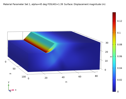
In the Model Builder window, expand the Results>Results: Material Set 1>Equivalent Plastic Strain 1 node, then click Surface 1.
2
In the Settings window for Surface, click to expand the Range section.
3
Select the Manual color range check box.
4
In the Maximum text field, type 0.15.
5
In the Equivalent Plastic Strain 1 toolbar, click  Plot.
Results: Material Set 2
In the Model Builder window, expand the Results>Results: Material Set 2 node.
Surface 1
1
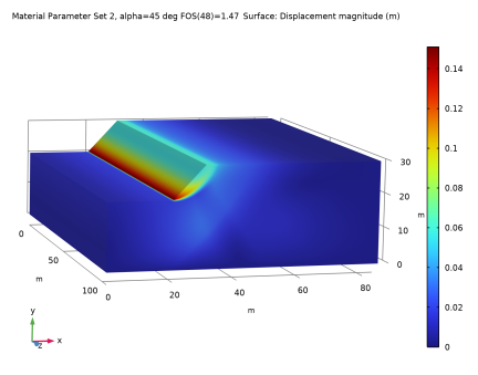
In the Model Builder window, expand the Results>Results: Material Set 2>Equivalent Plastic Strain 2 node, then click Surface 1.
2
In the Settings window for Surface, locate the Range section.
3
Select the Manual color range check box.
4
In the Maximum text field, type 0.08.
5
In the Equivalent Plastic Strain 2 toolbar, click  Plot.