
|
|
|
|
•
|
|
|
||||
|
•
|
|
•
|
|
•
|
In COMSOL Multiphysics, either the void ratio at reference pressure together with the saturation eref0, or the initial void ratio e0 are needed as a material property. For this example, an initial void ratio is provided as an input material property.
|
|
•
|
For the oedometer and triaxial tests, the compression index at current suction is independent of the suction, since suction values are held constant in Ref. 2. To achieve this, the weight parameter is set to zero. In COMSOL Multiphysics, the formula for the compression index at current suction is implemented in a different way, therefore, the weight parameter is set to one in order to achieve the same effect as shown in Ref. 2. In these cases the choice of the soil stiffness parameter does not matter.
|
|
•
|
The yield function and the plastic potential used in COMSOL Multiphysics is different than the expressions given in Ref. 2. The nonassociative parameter for the plastic potential is always set to one in COMSOL Multiphysics as compared to Ref. 2.
|
|
•
|
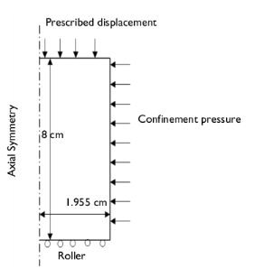
For the oedometer test, an initial stress of −2.97 MPa is applied in the radial and circumferential directions, while −0.18 MPa is applied in the axial direction.
|
|
•
|
Note that the reference pressure pref acts as an initial stress, therefore the values of the diagonal components of the in-situ stress tensor defined in the External Stress node are −2.87 MPa, −2.87 MPa, and −0.08 MPa.
|
|
•
|
During the loading stage of the oedometer test, the axial compressive stress is increased from 0.18 MPa to 19.77 MPa, and then decreased from 19.77 MPa to 1.00 MPa. Roller boundary conditions are applied on the bottom and side boundaries. The suction value is kept constant throughout the analysis.
|
|
•
|
For the uniaxial swelling test, an initial stress of −2.54 MPa is applied in the radial and circumferential directions, while −8.90 MPa is applied in the axial direction. The reference pressure pref acts as an initial stress, so the values of the diagonal components of the in-situ stress tensor in the External Stress node are -2.34 MPa, −2.34 MPa, and −8.70 MPa.
|
|
•
|
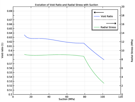
In the loading step of the uniaxial swelling test, the axial compressive stress is maintained constant at −8.90 MPa, while the suction is reduced from 101.5 MPa to 12.6 MPa. Roller boundary conditions are applied on the bottom and side boundaries.
|
|
•
|
For the triaxial test in isotropic compression, an initial hydrostatic stress of 1.1 MPa is applied. As the reference pressure pref acts as an initial stress, the values of the diagonal components of the in-situ stress tensor defined in the External Stress node are −1 MPa.
|
|
•
|
|
1
|
|
2
|
|
3
|
|
5
|
Click
|
|
6
|
|
7
|
Click
|
|
1
|
|
2
|
|
1
|
|
2
|
|
3
|
|
4
|
Browse to the model’s Application Libraries folder and double-click the file mechanical_modeling_of_bentonite_clay_oedometer_parameters.txt.
|
|
5
|
|
6
|
|
7
|
|
8
|
|
9
|
|
10
|
Browse to the model’s Application Libraries folder and double-click the file mechanical_modeling_of_bentonite_clay_uniaxial_swelling_parameters.txt.
|
|
11
|
|
12
|
|
13
|
|
14
|
Browse to the model’s Application Libraries folder and double-click the file mechanical_modeling_of_bentonite_clay_triaxial_parameters.txt.
|
|
15
|
|
16
|
|
17
|
|
18
|
Browse to the model’s Application Libraries folder and double-click the file mechanical_modeling_of_bentonite_clay_constrained_swelling_parameters.txt.
|
|
1
|
|
2
|
|
3
|
|
4
|
|
5
|
|
1
|
|
2
|
In the Settings window for Solid Mechanics, type Solid Mechanics [Oedometer Test] in the Label text field.
|
|
1
|
|
3
|
In the Settings window for Elastoplastic Soil Material, locate the Elastoplastic Soil Material section.
|
|
4
|
|
5
|
|
6
|
|
7
|
|
8
|
|
9
|
|
1
|
|
2
|
|
3
|
|
4
|
From the list, choose Symmetric.
|
|
5
|
|
1
|
|
1
|
|
2
|
|
3
|
|
5
|
|
6
|
In the Function table, enter the following settings:
|
|
1
|
|
3
|
|
4
|
|
5
|
|
1
|
|
3
|
|
4
|
|
5
|
|
6
|
|
7
|
In the Show More Options dialog box, in the tree, select the check box for the node Physics>Equation-Based Contributions.
|
|
8
|
Click OK.
|
|
1
|
|
2
|
|
4
|
|
5
|
|
6
|
Click
|
|
7
|
|
8
|
Click OK.
|
|
9
|
|
10
|
|
11
|
|
12
|
Click
|
|
13
|
|
14
|
Click OK.
|
|
1
|
|
2
|
|
3
|
|
5
|
|
6
|
In the Function table, enter the following settings:
|
|
1
|
|
2
|
In the Settings window for Solid Mechanics, type Solid Mechanics [Uniaxial Swelling Test] in the Label text field.
|
|
1
|
|
3
|
In the Settings window for Elastoplastic Soil Material, locate the Elastoplastic Soil Material section.
|
|
4
|
|
5
|
|
6
|
|
7
|
|
8
|
|
9
|
|
1
|
|
2
|
|
3
|
|
4
|
From the list, choose Symmetric.
|
|
5
|
|
1
|
|
1
|
|
3
|
|
4
|
|
5
|
|
1
|
|
2
|
|
4
|
|
5
|
|
6
|
Click
|
|
7
|
|
8
|
Click OK.
|
|
9
|
|
10
|
|
11
|
|
12
|
Click
|
|
13
|
|
14
|
Click OK.
|
|
1
|
|
2
|
In the Settings window for Solid Mechanics, type Solid Mechanics [Triaxial Test] in the Label text field.
|
|
1
|
|
3
|
In the Settings window for Elastoplastic Soil Material, locate the Elastoplastic Soil Material section.
|
|
4
|
|
5
|
|
6
|
|
7
|
|
8
|
|
9
|
|
1
|
|
2
|
|
3
|
|
4
|
|
1
|
|
1
|
|
3
|
|
4
|
|
5
|
|
1
|
|
2
|
In the Settings window for Solid Mechanics, type Solid Mechanics [Constrained Swelling Test] in the Label text field.
|
|
1
|
|
3
|
In the Settings window for Elastoplastic Soil Material, locate the Elastoplastic Soil Material section.
|
|
4
|
|
5
|
|
6
|
|
7
|
|
8
|
|
9
|
|
1
|
|
1
|
In the Model Builder window, under Component 1 (comp1) right-click Definitions and choose Variables.
|
|
2
|
|
1
|
In the Model Builder window, under Component 1 (comp1) right-click Materials and choose Blank Material.
|
|
2
|
|
3
|
|
1
|
|
2
|
|
3
|
|
4
|
|
5
|
|
1
|
|
2
|
|
3
|
|
4
|
|
5
|
|
6
|
|
7
|
|
8
|
|
9
|
|
1
|
|
2
|
|
1
|
|
2
|
|
3
|
Click
|
|
4
|
|
5
|
Click
|
|
1
|
|
2
|
|
3
|
In the table, clear the Solve for check boxes for Solid Mechanics [Uniaxial Swelling Test] (solid2), Solid Mechanics [Triaxial Test] (solid3), and Solid Mechanics [Constrained Swelling Test] (solid4).
|
|
4
|
|
5
|
Click
|
|
1
|
|
2
|
|
3
|
In the Model Builder window, expand the Study [Oedometer Test]>Solver Configurations>Solution 1 (sol1)>Dependent Variables 1 node, then click State variable disp1 (comp1.ODE1).
|
|
4
|
|
5
|
|
6
|
|
7
|
In the Model Builder window, expand the Study [Oedometer Test]>Solver Configurations>Solution 1 (sol1)>Stationary Solver 1 node, then click Fully Coupled 1.
|
|
8
|
|
9
|
|
10
|
|
11
|
|
1
|
|
2
|
|
3
|
|
1
|
|
2
|
|
3
|
|
4
|
Click
|
|
1
|
|
2
|
|
3
|
In the table, clear the Solve for check boxes for Solid Mechanics [Oedometer Test] (solid), Solid Mechanics [Triaxial Test] (solid3), and Solid Mechanics [Constrained Swelling Test] (solid4).
|
|
4
|
|
5
|
Click
|
|
7
|
|
1
|
|
2
|
|
3
|
|
1
|
|
2
|
|
3
|
|
4
|
Click
|
|
1
|
|
2
|
|
3
|
In the table, clear the Solve for check boxes for Solid Mechanics [Oedometer Test] (solid), Solid Mechanics [Uniaxial Swelling Test] (solid2), and Solid Mechanics [Constrained Swelling Test] (solid4).
|
|
4
|
|
5
|
Click
|
|
1
|
|
2
|
|
3
|
In the Model Builder window, expand the Study [Triaxial Test]>Solver Configurations>Solution 7 (sol7)>Stationary Solver 1 node, then click Fully Coupled 1.
|
|
4
|
|
5
|
|
6
|
|
7
|
|
1
|
|
2
|
|
3
|
|
1
|
|
2
|
|
3
|
|
4
|
Click
|
|
1
|
|
2
|
|
3
|
In the table, clear the Solve for check boxes for Solid Mechanics [Oedometer Test] (solid), Solid Mechanics [Uniaxial Swelling Test] (solid2), and Solid Mechanics [Triaxial Test] (solid3).
|
|
4
|
|
5
|
Click
|
|
1
|
|
2
|
|
3
|
In the Model Builder window, expand the Study [Constrained Swelling Test]>Solver Configurations>Solution 10 (sol10)>Stationary Solver 1 node, then click Fully Coupled 1.
|
|
4
|
|
5
|
|
6
|
|
1
|
|
2
|
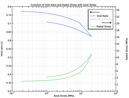
In the Settings window for 1D Plot Group, type Evolution of Void Ratio and Radial Stress with Axial Stress [Oedometer Test] in the Label text field.
|
|
3
|
|
4
|
|
5
|
Click to collapse the Title section. Locate the Plot Settings section. Select the Two y-axes check box.
|
|
6
|
|
7
|
Select the Secondary y-axis label check box. In the associated text field, type Radial Stress (MPa).
|
|
8
|
|
9
|
|
10
|
|
11
|
|
12
|
|
13
|
|
14
|
|
15
|
|
1
|
Right-click Evolution of Void Ratio and Radial Stress with Axial Stress [Oedometer Test] and choose Point Graph.
|
|
3
|
|
4
|
|
5
|
|
6
|
|
7
|
|
8
|
|
9
|
|
1
|
|
2
|
|
3
|
|
4
|
|
5
|
|
6
|
Locate the Legends section. In the table, enter the following settings:
|
|
7
|
In the Evolution of Void Ratio and Radial Stress with Axial Stress [Oedometer Test] toolbar, click
|
|
1
|
|
2
|
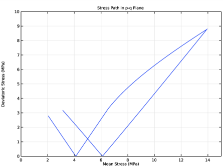
In the Settings window for 1D Plot Group, type Stress Path in p-q Plane [Oedometer Test] in the Label text field.
|
|
3
|
|
4
|
|
5
|
|
6
|
|
7
|
|
8
|
|
9
|
|
10
|
|
11
|
|
12
|
|
1
|
|
3
|
|
4
|
|
5
|
|
6
|
|
7
|
|
8
|
|
9
|
|
1
|
|
2
|
In the Settings window for 1D Plot Group, type Evolution of Void Ratio and Radial Stress with Suction [Uniaxial Swelling Test] in the Label text field.
|
|
3
|
Locate the Data section. From the Dataset list, choose Study [Uniaxial Swelling Test]/Solution 4 (sol4).
|
|
4
|
|
5
|
|
6
|
Click to collapse the Title section. Locate the Plot Settings section. Select the Two y-axes check box.
|
|
7
|
|
8
|
Select the Secondary y-axis label check box. In the associated text field, type Radial Stress (MPa).
|
|
9
|
|
10
|
|
11
|
|
12
|
|
13
|
|
14
|
|
15
|
|
1
|
Right-click Evolution of Void Ratio and Radial Stress with Suction [Uniaxial Swelling Test] and choose Point Graph.
|
|
3
|
|
4
|
|
5
|
|
6
|
|
7
|
|
8
|
|
9
|
|
1
|
|
2
|
|
3
|
|
4
|
|
5
|
|
6
|
Locate the Legends section. In the table, enter the following settings:
|
|
7
|
In the Evolution of Void Ratio and Radial Stress with Suction [Uniaxial Swelling Test] toolbar, click
|
|
1
|
|
2
|
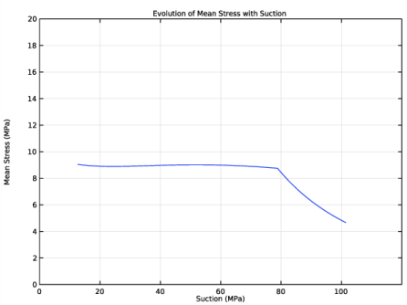
In the Settings window for 1D Plot Group, type Evolution of Mean Stress with Suction [Uniaxial Swelling Test] in the Label text field.
|
|
3
|
Locate the Data section. From the Dataset list, choose Study [Uniaxial Swelling Test]/Solution 4 (sol4).
|
|
4
|
|
5
|
|
6
|
|
7
|
|
8
|
|
9
|
|
10
|
|
11
|
|
12
|
|
13
|
|
1
|
|
3
|
|
4
|
|
5
|
|
6
|
|
7
|
|
8
|
|
9
|
|
1
|
|
2
|
In the Settings window for 1D Plot Group, type Stress Path in p-q Plane [Uniaxial Swelling Test] in the Label text field.
|
|
3
|
Locate the Data section. From the Dataset list, choose Study [Uniaxial Swelling Test]/Solution 4 (sol4).
|
|
4
|
|
5
|
|
6
|
|
7
|
|
8
|
|
9
|
|
10
|
|
11
|
|
12
|
|
13
|
|
1
|
|
3
|
|
4
|
|
5
|
|
6
|
|
7
|
|
8
|
|
9
|
|
1
|
|
2
|
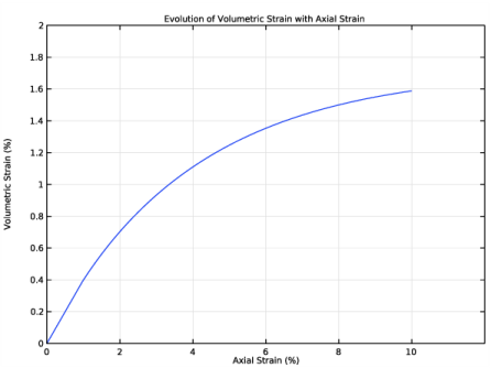
In the Settings window for 1D Plot Group, type Evolution of Volumetric Strain with Axial Strain [Triaxial Test] in the Label text field.
|
|
3
|
|
4
|
|
5
|
|
6
|
|
7
|
|
8
|
|
9
|
|
10
|
|
11
|
|
12
|
|
13
|
|
1
|
Right-click Evolution of Volumetric Strain with Axial Strain [Triaxial Test] and choose Point Graph.
|
|
3
|
|
4
|
|
5
|
|
6
|
|
7
|
|
8
|
|
9
|
|
1
|
|
2
|
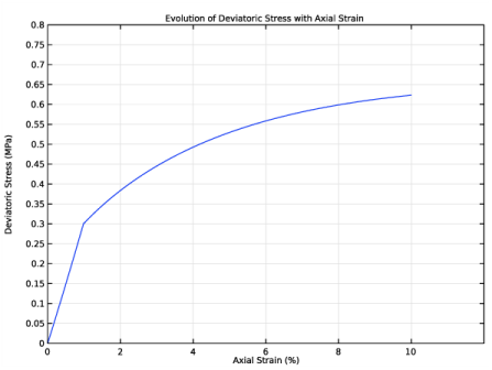
In the Settings window for 1D Plot Group, type Evolution of Deviatoric Stress with Axial Strain [Triaxial Test] in the Label text field.
|
|
3
|
|
4
|
|
5
|
|
6
|
|
7
|
|
8
|
|
9
|
|
10
|
|
11
|
|
12
|
|
13
|
|
1
|
Right-click Evolution of Deviatoric Stress with Axial Strain [Triaxial Test] and choose Point Graph.
|
|
3
|
|
4
|
|
5
|
|
6
|
|
7
|
|
8
|
|
9
|
|
1
|
|
2
|
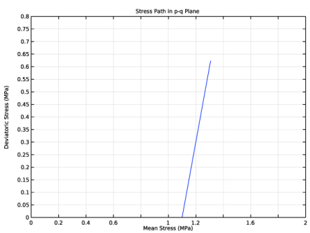
In the Settings window for 1D Plot Group, type Stress Path in p-q Plane [Triaxial Test] in the Label text field.
|
|
3
|
|
4
|
|
5
|
|
6
|
|
7
|
|
8
|
|
9
|
|
10
|
|
11
|
|
12
|
|
13
|
|
1
|
|
3
|
|
4
|
|
5
|
|
6
|
|
7
|
|
8
|
|
9
|
|
1
|
|
2
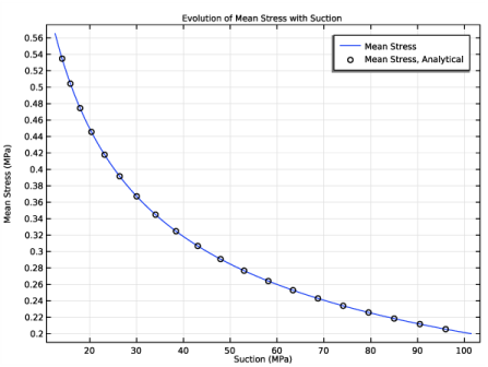
|
In the Settings window for 1D Plot Group, type Evolution of Mean Stress with Suction [Constrained Swelling Test] in the Label text field.
|
|
3
|
|
4
|
|
5
|
Locate the Data section. From the Dataset list, choose Study [Constrained Swelling Test]/Solution 10 (sol10).
|
|
6
|
|
7
|
|
8
|
|
1
|
Right-click Evolution of Mean Stress with Suction [Constrained Swelling Test] and choose Point Graph.
|
|
3
|
|
4
|
|
5
|
|
6
|
|
7
|
|
8
|
|
9
|
Click to expand the Coloring and Style section. Locate the Legends section. Select the Show legends check box.
|
|
10
|
|
1
|
|
2
|
|
3
|
|
4
|
Locate the Legends section. In the table, enter the following settings:
|
|
5
|
|
6
|
|
7
|
|
8
|
|
9
|
|
10
|
|
1
|
|
2
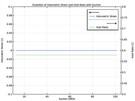
|
In the Settings window for 1D Plot Group, type Evolution of Volumetric Strain and Void Ratio with Suction [Constrained Swelling Test] in the Label text field.
|
|
3
|
Locate the Data section. From the Dataset list, choose Study [Constrained Swelling Test]/Solution 10 (sol10).
|
|
4
|
|
5
|
|
6
|
|
7
|
|
8
|
|
9
|
|
10
|
|
11
|
|
12
|
|
13
|
|
14
|
|
15
|
|
16
|
|
1
|
Right-click Evolution of Volumetric Strain and Void Ratio with Suction [Constrained Swelling Test] and choose Point Graph.
|
|
3
|
|
4
|
|
5
|
|
6
|
|
7
|
|
8
|
|
9
|
|
1
|
|
2
|
|
3
|
|
4
|
|
5
|
Locate the Legends section. In the table, enter the following settings:
|
|
1
|
In the Model Builder window, collapse the Results>Evolution of Volumetric Strain and Void Ratio with Suction [Constrained Swelling Test] node.
|
|
2
|
In the Model Builder window, click Evolution of Volumetric Strain and Void Ratio with Suction [Constrained Swelling Test].
|
|
3
|
In the Evolution of Volumetric Strain and Void Ratio with Suction [Constrained Swelling Test] toolbar, click
|