You are viewing the documentation for an older COMSOL version. The latest version is available here.
PDF

Isotropic Compression with Modified Cam-Clay Material Model
Introduction
Isotropic compression is a common material test for soils. In this example, the Modified Cam-Clay (MCC) soil model is examined; in particular the relation between the void ratio and the logarithm of the hydrostatic pressure or mean stress is studied.
In COMSOL Multiphysics, several soil plasticity material models are implemented. With particular choices of parameters, some of these can be reduced to the MCC model. For example, the Extended Barcelona Basic model (BBMx) with zero suction reduces to the Modified Cam-Clay model. By setting the initial structural strength and the additional void ratio to zero and the plastic potential shape parameter to two, the Modified Structured Cam-Clay (MSCC) model reduces to the MCC model. With these choices of material parameters, we can verify that the BBMx and MSCC models replicate the behavior of the MCC model.
Model Definition
In this example, the test specimen is a cylindrical soil sample of 10 cm in diameter and 10 cm in height, see Figure 1. Due to the symmetry, the model is solved in 2D axisymmetry. A boundary load produces isotropic compression conditions.
Figure 1: Dimensions, boundary conditions, and boundary loads for the isotropic compression test.
Modified Cam-Clay Material Properties
ρ
κ
λ
eref
pref
pc0
Extended Barcelona basic Material Properties
Common material properties are the same as for the MCC model. Properties that are specific to the BBMx are listed in Table 2.
σ
κs
λs
bs
sy0
Note that material parameters related to the suction are chosen arbitrarily and does not affect the results since the suction is set to zero.
Modified structured Cam-Clay Material Properties
The material parameters in common for the MSCC and MCC models are set identical.The properties that are specific to the MSCC model are listed in Table 3.
pbi
ζ
Δei
dv
ds
εdcp
Note that material parameters related to the structuring are chosen arbitrarily and does not affect the results since the structure strength will be set to zero in the Elastoplastic Soil feature.
Constraints and Loads
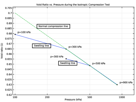
The boundary load is applied in three steps: First the pressure increases from 0.5p0 to 3p0. Next, the pressure is reduced to 1.5p0, and finally the pressure increases again up to 4p0.
In order to reproduce the analytical results of Ref. 1, the load is controlled in a parametric analysis.
Results and Discussion
The relation between void ratio and pressure is shown in Figure 2. Note that the pressure is plotted on a logarithmic scale.
Figure 2: Void ratio as a function of the pressure in an isotropic compression test.
For the pressures from 100 kPa to 300 kPa, the curve follows the slope defined by the swelling index κ. Once the consolidation pressure is reached (pc0 = 300 kPa), the soil behaves plastically, and the curve follows the slope defined by the compression index λ. During the unloading and reloading of the soil (between the parameters 0.4 and 0.8), the curve in Figure 2 follows the elastic slope defined by the swelling index κ. Finally, the soil is compressed between the parameters 0.8 and 1, and it undergoes plastic deformation until it reaches its final stage at a void ratio e0 = 0.630 at p = 900 kPa.
Figure 2 reproduces characteristic curves called the Normal Compression Line (NCL) and the Swelling Line (or Unloading/Reloading Line URL). The NCL has a slope defined by the compression index λ, and at p = pref on the NCL the void ratio is e = eref.
Figure 3: Void ratio versus pressure in the isotropic compression test for all three material models.
Figure 3 shows the variation in the void ratio with applied pressure for all three models. The behavior predicted is the same for all soil models, which verifies the correctness of the BBMx model for the case of saturated soils and that of the MSCC model for destructured soils.
Once the stress level reaches the MCC ellipse in stress space, (p = pc0, parameter para = 0.2), the soil starts deforming plastically. Isotropic hardening expands the major semi-axis of the ellipse, with the expansion determined by the increase in consolidation pressure, see Figure 4. During the unloading–reloading steps (between parameter values 0.4 and 0.8), the consolidation pressure is kept constant.
The changes in consolidation pressure with respect to the boundary load is identical for all three material models, as expected.
Figure 4: Increase in consolidation pressure due to isotropic hardening.
Reference
1. W.F. Chen and E. Mizuno, Nonlinear Analysis in Soil Mechanics, Elsevier, 1990.
Application Library path: Geomechanics_Module/Verification_Examples/isotropic_compression
Modeling Instructions
From the File menu, choose New.
New
In the New window, click  Model Wizard.
Model Wizard
1
In the Model Wizard window, click  2D Axisymmetric.
2
In the Select Physics tree, select Structural Mechanics>Solid Mechanics (solid).
3
Click Add.
4
Global Definitions
Parameters 1
1
In the Model Builder window, under Global Definitions click Parameters 1.
2
In the Settings window for Parameters, locate the Parameters section.
3
Boundary Load
1
In the Home toolbar, click  Functions and choose Global>Interpolation.
2
In the Settings window for Interpolation, locate the Definition section.
3
In the Function name text field, type Pressure.
4
In the Label text field, type Boundary Load.
5
Locate the Definition section. In the table, enter the following settings:
6
Locate the Units section. In the Argument table, enter the following settings:
7
In the Function table, enter the following settings:
8
An interpolation function is used to define the boundary load. First, a pressure of 2*p0 is applied. Next, the load is reduced to p0 followed by a reloading to 2*p0 and finally an increase up to 4*p0.
Geometry 1
Rectangle 1 (r1)
1
In the Geometry toolbar, click  Rectangle.
2
In the Settings window for Rectangle, locate the Size and Shape section.
3
In the Width text field, type 5[cm].
4
In the Height text field, type 10[cm].
Array 1 (arr1)
1
In the Geometry toolbar, click  Transforms and choose Array.
2
3
In the Settings window for Array, locate the Size section.
4
In the z size text field, type 3.
5
Locate the Displacement section. In the z text field, type 15[cm].
6
Click  Build All Objects.
7
Click the  Zoom Extents button in the Graphics toolbar.
Add the three different Elastoplastic Soil material models. Start with the MCC model.
Solid Mechanics (solid)
Modified Cam-Clay Model (MCC)
1
In the Model Builder window, under Component 1 (comp1) right-click Solid Mechanics (solid) and choose Material Models>Elastoplastic Soil Material.
2
In the Settings window for Elastoplastic Soil Material, type Modified Cam-Clay Model (MCC) in the Label text field.
3
4
Locate the Elastoplastic Soil Material section. From the Specify list, choose Shear modulus.
5
From the M list, choose Match to Mohr-Coulomb criterion.
6
In the pc0 text field, type 300[kPa].
Next, add an BBMx model with zero suction in order to replicate the MCC behavior.
Extended Barcelona Basic Model (BBMx)
1
In the Model Builder window, right-click Modified Cam-Clay Model (MCC) and choose Duplicate.
2
In the Settings window for Elastoplastic Soil Material, type Extended Barcelona Basic Model (BBMx) in the Label text field.
3
Locate the Domain Selection section. Click  Clear Selection.
4
5
Locate the Elastoplastic Soil Material section. From the Material model list, choose Extended Barcelona Basic.
6
In the s text field, type 0.
Last, add a MSCC model. Set the initial structural strength and the additional void ratio to zero. Also, set the plastic potential shape parameter to 2.
Modified Structured Cam-Clay Model (MSCC)
1
In the Model Builder window, right-click Modified Cam-Clay Model (MCC) and choose Duplicate.
2
In the Settings window for Elastoplastic Soil Material, type Modified Structured Cam-Clay Model (MSCC) in the Label text field.
3
Locate the Domain Selection section. Click  Clear Selection.
4
5
Locate the Elastoplastic Soil Material section. From the Material model list, choose Modified Structured Cam-Clay.
6
From the M list, choose Match to Mohr-Coulomb criterion.
7
From the pbi list, choose User defined. From the ζ list, choose User defined. In the associated text field, type 2.
8
From the Δei list, choose User defined.
Add one Material feature for each of the three models. Note that the material properties in common should be kept the same between all models. The parameters unique to the BBMx and MSCC models are set arbitrarily, as they have no influence on the solution because of the settings chosen in the corresponding Elastoplastic Soil Material nodes under Solid Mechanics.
Materials
Modified Cam-Clay Material
1
In the Model Builder window, under Component 1 (comp1) right-click Materials and choose Blank Material.
2
In the Settings window for Material, type Modified Cam-Clay Material in the Label text field.
3
Locate the Geometric Entity Selection section. Click  Clear Selection.
4
5
Locate the Material Contents section. In the table, enter the following settings:
Extended Barcelona Basic Material
1
In the Model Builder window, under Component 1 (comp1)>Materials right-click Modified Cam-Clay Material (mat1) and choose Duplicate.
2
In the Settings window for Material, type Extended Barcelona Basic Material in the Label text field.
3
Locate the Geometric Entity Selection section. Click  Clear Selection.
4
5
Locate the Material Contents section. In the table, enter the following settings:
Modified Structured Cam-Clay Material
1
In the Model Builder window, under Component 1 (comp1)>Materials right-click Extended Barcelona Basic Material  (mat2) and choose Duplicate.
2
In the Settings window for Material, type Modified Structured Cam-Clay Material in the Label text field.
3
Locate the Geometric Entity Selection section. Click  Clear Selection.
4
5
Locate the Material Contents section. In the table, enter the following settings:
Use the Test Material feature to carry out isotropic compression tests on the three different material models.
Solid Mechanics (solid)
Test Material [Modified Cam-Clay Model]
1
In the Physics toolbar, click  Global and choose Test Material.
2
In the Settings window for Test Material, type Test Material [Modified Cam-Clay Model] in the Label text field.
3
4
Locate the Material Tests section. In the Np text field, type 100.
5
From the Test setup list, choose User defined.
6
From the Test control list, choose Force driven.
7
Find the Tests subsection. Clear the Uniaxial test check box.
8
Select the Isotropic test check box.
9
In the p text field, type -Pressure(para).
10
Click Auto Test Setup in the upper-right corner of the Material Tests section. From the menu, choose Set up Tests.
Test Material [Extended Barcelona Basic Model]
1
In the Model Builder window, right-click Test Material [Modified Cam-Clay Model] and choose Duplicate.
2
In the Settings window for Test Material, type Test Material [Extended Barcelona Basic Model] in the Label text field.
3
Locate the Domain Selection section. Click  Clear Selection.
4
5
Click Auto Test Setup in the upper-right corner of the Material Tests section. From the menu, choose Set up Tests.
Test Material [Modified Structured Cam-Clay Model]
1
In the Model Builder window, right-click Test Material [Modified Cam-Clay Model] and choose Duplicate.
2
In the Settings window for Test Material, type Test Material [Modified Structured Cam-Clay Model] in the Label text field.
3
Locate the Domain Selection section. Click  Clear Selection.
4
5
Click Auto Test Setup in the upper-right corner of the Material Tests section. From the menu, choose Set up Tests.
Results
In the Model Builder window, expand the Results>Datasets node.
Study: Test Material [Extended Barcelona Basic Model]/Solution 1a (8) (solidtm2sol1), Study: Test Material [Extended Barcelona Basic Model]/Solution 1a (9) (solidtm2sol1), Study: Test Material [Extended Barcelona Basic Model]/Solution 2 (5) (solidtm2sol), Study: Test Material [Extended Barcelona Basic Model]/Solution 2 (6) (solidtm2sol), Study: Test Material [Extended Barcelona Basic Model]/Solution 2 (7) (solidtm2sol), Study: Test Material [Modified Cam-Clay Model]/Solution (1) (solidtm1sol), Study: Test Material [Modified Cam-Clay Model]/Solution (2) (solidtm1sol), Study: Test Material [Modified Cam-Clay Model]/Solution 1 (3) (solidtm1sol1), Study: Test Material [Modified Structured Cam-Clay Model]/Solution 1b (15) (solidtm3sol1), Study: Test Material [Modified Structured Cam-Clay Model]/Solution 1b (16) (solidtm3sol1), Study: Test Material [Modified Structured Cam-Clay Model]/Solution 1b (17) (solidtm3sol1), Study: Test Material [Modified Structured Cam-Clay Model]/Solution 3 (11) (solidtm3sol), Study: Test Material [Modified Structured Cam-Clay Model]/Solution 3 (12) (solidtm3sol), Study: Test Material [Modified Structured Cam-Clay Model]/Solution 3 (13) (solidtm3sol), Study: Test Material [Modified Structured Cam-Clay Model]/Solution 3 (14) (solidtm3sol)
1
In the Model Builder window, under Results>Datasets, Ctrl-click to select Study: Test Material [Modified Cam-Clay Model]/Solution (1) (solidtm1sol), Study: Test Material [Modified Cam-Clay Model]/Solution (2) (solidtm1sol), Study: Test Material [Modified Cam-Clay Model]/Solution 1 (3) (solidtm1sol1), Study: Test Material [Extended Barcelona Basic Model]/Solution 2 (5) (solidtm2sol), Study: Test Material [Extended Barcelona Basic Model]/Solution 2 (6) (solidtm2sol), Study: Test Material [Extended Barcelona Basic Model]/Solution 2 (7) (solidtm2sol), Study: Test Material [Extended Barcelona Basic Model]/Solution 1a (8) (solidtm2sol1), Study: Test Material [Extended Barcelona Basic Model]/Solution 1a (9) (solidtm2sol1), Study: Test Material [Modified Structured Cam-Clay Model]/Solution 3 (11) (solidtm3sol), Study: Test Material [Modified Structured Cam-Clay Model]/Solution 3 (12) (solidtm3sol), Study: Test Material [Modified Structured Cam-Clay Model]/Solution 3 (13) (solidtm3sol), Study: Test Material [Modified Structured Cam-Clay Model]/Solution 3 (14) (solidtm3sol), Study: Test Material [Modified Structured Cam-Clay Model]/Solution 1b (15) (solidtm3sol1), Study: Test Material [Modified Structured Cam-Clay Model]/Solution 1b (16) (solidtm3sol1), and Study: Test Material [Modified Structured Cam-Clay Model]/Solution 1b (17) (solidtm3sol1).
2
Void Ratio (MCC)
1
In the Home toolbar, click  Add Plot Group and choose 1D Plot Group.
2
In the Settings window for 1D Plot Group, type Void Ratio (MCC) in the Label text field.
3
Locate the Data section. From the Dataset list, choose Study: Test Material [Modified Cam-Clay Model]/Solution 1 (solidtm1sol1).
4
Click to expand the Title section. From the Title type list, choose Manual.
5
In the Title text area, type Void Ratio vs. Pressure during the Isotropic Compression Test.
6
Locate the Plot Settings section.
7
Select the x-axis label check box. In the associated text field, type Pressure (kPa).
8
Select the y-axis label check box. In the associated text field, type Void ratio (1).
9
Locate the Axis section. Select the Manual axis limits check box.
10
In the x minimum text field, type 95.
11
In the x maximum text field, type 1300.
12
In the y minimum text field, type 0.62.
13
In the y maximum text field, type 0.706.
14
Set the x-axis in the e vs. p plot to logarithmic.
15
Select the x-axis log scale check box.
Point Graph 1
1
Right-click Void Ratio (MCC) and choose Point Graph.
2
3
In the Settings window for Point Graph, click Replace Expression in the upper-right corner of the y-Axis Data section. From the menu, choose Component: Test Material [Modified Cam-Clay Model] (solidtm1comp)>Solid Mechanics>Soil material properties>Modified Cam-Clay>solid1.epsm1.evoid - Void ratio.
4
Click Replace Expression in the upper-right corner of the x-Axis Data section. From the menu, choose Component: Test Material [Modified Cam-Clay Model] (solidtm1comp)>Solid Mechanics>Stress>solid1.pm - Pressure - N/m².
5
Locate the x-Axis Data section. From the Unit list, choose kPa.
6
In the Void Ratio (MCC) toolbar, click  Plot.
Annotation 1
1
In the Model Builder window, right-click Void Ratio (MCC) and choose Annotation.
2
In the Settings window for Annotation, locate the Data section.
3
From the Dataset list, choose Study: Test Material [Modified Cam-Clay Model]/Solution 1 (solidtm1sol1).
4
From the Parameter value (para) list, choose 0.
5
Locate the Annotation section. In the Text text field, type p=eval(at3(0,0,0,solid1.pm), kPa) kPa.
6
From the Geometry level list, choose Global.
7
Locate the Position section. In the X text field, type at3(0,0,0,solid1.pm)/1000.
8
In the Y text field, type at3(0,0,0,solid1.epsm1.evoid).
9
Click to expand the Advanced section. In the Expression precision text field, type 3.
10
Locate the Coloring and Style section. From the Anchor point list, choose Lower left.
Annotation 2
1
Right-click Annotation 1 and choose Duplicate.
2
In the Settings window for Annotation, locate the Data section.
3
From the Parameter value (para) list, choose 0.2.
Annotation 3
1
Right-click Annotation 2 and choose Duplicate.
2
In the Settings window for Annotation, locate the Data section.
3
From the Parameter value (para) list, choose 0.4.
Annotation 4
1
Right-click Annotation 3 and choose Duplicate.
2
In the Settings window for Annotation, locate the Data section.
3
From the Parameter value (para) list, choose 0.6.
4
Locate the Coloring and Style section. From the Anchor point list, choose Lower right.
Annotation 5
1
Right-click Annotation 4 and choose Duplicate.
2
In the Settings window for Annotation, locate the Data section.
3
From the Parameter value (para) list, choose 1.
4
Locate the Coloring and Style section. From the Anchor point list, choose Lower left.
Point Graph 2
1
In the Model Builder window, under Results>Void Ratio (MCC) right-click Point Graph 1 and choose Duplicate.
2
In the Settings window for Point Graph, locate the y-Axis Data section.
3
In the Expression text field, type solid1.epsm1.evoidref-solid1.epsm1.lambdaComp*log(solid1.epsm1.p/solid1.epsm1.pref).
4
Click to expand the Coloring and Style section. Find the Line style subsection. From the Line list, choose Dashed.
Void Ratio (MCC)
In the Model Builder window, click Void Ratio (MCC).
Table Annotation 1
1
In the Void Ratio (MCC) toolbar, click  More Plots and choose Table Annotation.
2
In the Settings window for Table Annotation, locate the Data section.
3
From the Source list, choose Local table.
4
5
Locate the Coloring and Style section. Clear the Show point check box.
6
Select the Show frame check box.
7
In the Void Ratio (MCC) toolbar, click  Plot.
Void Ratio (MCC), Numerical Vs. Analytical
1
In the Home toolbar, click  Add Plot Group and choose 1D Plot Group.
2
In the Settings window for 1D Plot Group, type Void Ratio (MCC), Numerical Vs. Analytical in the Label text field.
3
Locate the Data section. From the Dataset list, choose Study: Test Material [Modified Cam-Clay Model]/Solution 1 (solidtm1sol1).
4
Locate the Title section. From the Title type list, choose Manual.
5
In the Title text area, type Void Ratio vs. Pressure during the Isotropic Compression Test.
6
Locate the Plot Settings section.
7
Select the x-axis label check box. In the associated text field, type Pressure (kPa).
8
Select the y-axis label check box. In the associated text field, type Void ratio (1).
9
Locate the Axis section. Select the x-axis log scale check box.
Point Graph 1
1
Right-click Void Ratio (MCC), Numerical Vs. Analytical and choose Point Graph.
2
3
In the Settings window for Point Graph, click Replace Expression in the upper-right corner of the y-Axis Data section. From the menu, choose Component: Test Material [Modified Cam-Clay Model] (solidtm1comp)>Solid Mechanics>Soil material properties>Modified Cam-Clay>solid1.epsm1.evoid - Void ratio.
4
Click Replace Expression in the upper-right corner of the x-Axis Data section. From the menu, choose Component: Test Material [Modified Cam-Clay Model] (solidtm1comp)>Solid Mechanics>Stress>solid1.pm - Pressure - N/m².
5
Locate the x-Axis Data section. From the Unit list, choose kPa.
6
From the Unit list, choose kPa.
7
Click to expand the Legends section. Select the Show legends check box.
8
From the Legends list, choose Manual.
9
Point Graph 2
1
Right-click Point Graph 1 and choose Duplicate.
2
In the Settings window for Point Graph, locate the y-Axis Data section.
3
In the Expression text field, type solid1.epsm1.evoidref-(solid1.epsm1.lambdaComp-solid1.epsm1.kappaSwelling)*log(solid1.epsm1.pc/solid1.epsm1.pref)-solid1.epsm1.kappaSwelling*log(solid1.epsm1.p/solid1.epsm1.pref).
4
Locate the Coloring and Style section. Find the Line style subsection. From the Line list, choose Dashed.
5
Locate the Legends section. In the table, enter the following settings:
6
In the Void Ratio (MCC), Numerical Vs. Analytical toolbar, click  Plot.
Void Ratio, MCC vs. BBMx vs. MSCC
1
In the Home toolbar, click  Add Plot Group and choose 1D Plot Group.
2
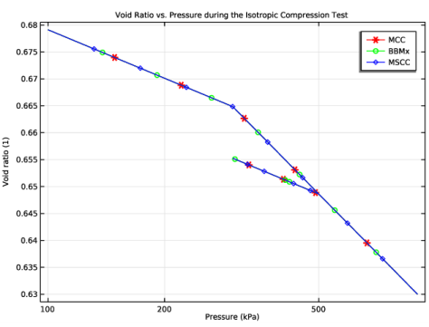
In the Settings window for 1D Plot Group, type Void Ratio, MCC vs. BBMx vs. MSCC in the Label text field.
3
Locate the Data section. From the Dataset list, choose Study: Test Material [Modified Cam-Clay Model]/Solution 1 (solidtm1sol1).
4
Locate the Title section. From the Title type list, choose Manual.
5
In the Title text area, type Void Ratio vs. Pressure during the Isotropic Compression Test.
6
Locate the Plot Settings section.
7
Select the x-axis label check box. In the associated text field, type Pressure (kPa).
8
Select the y-axis label check box. In the associated text field, type Void ratio (1).
9
Locate the Axis section. Select the x-axis log scale check box.
Point Graph 1
1
Right-click Void Ratio, MCC vs. BBMx vs. MSCC and choose Point Graph.
2
3
In the Settings window for Point Graph, click Replace Expression in the upper-right corner of the y-Axis Data section. From the menu, choose Component: Test Material [Modified Cam-Clay Model] (solidtm1comp)>Solid Mechanics>Soil material properties>Modified Cam-Clay>solid1.epsm1.evoid - Void ratio.
4
Click Replace Expression in the upper-right corner of the x-Axis Data section. From the menu, choose Component: Test Material [Modified Cam-Clay Model] (solidtm1comp)>Solid Mechanics>Stress>solid1.pm - Pressure - N/m².
5
Locate the x-Axis Data section. From the Unit list, choose kPa.
6
Locate the Coloring and Style section. From the Color list, choose Red.
7
Find the Line markers subsection. From the Marker list, choose Asterisk.
8
From the Positioning list, choose Interpolated.
9
Locate the Legends section. Select the Show legends check box.
10
From the Legends list, choose Manual.
11
Point Graph 2
1
In the Model Builder window, right-click Void Ratio, MCC vs. BBMx vs. MSCC and choose Point Graph.
2
In the Settings window for Point Graph, locate the Data section.
3
From the Dataset list, choose Study: Test Material [Extended Barcelona Basic Model]/Solution 1a (solidtm2sol1).
4
5
Click Replace Expression in the upper-right corner of the y-Axis Data section. From the menu, choose Component: Test Material [Extended Barcelona Basic Model] (solidtm2comp)>Solid Mechanics>Soil material properties>Extended Barcelona Basic>solid2.epsm2.evoid - Void ratio.
6
Click Replace Expression in the upper-right corner of the x-Axis Data section. From the menu, choose Component: Test Material [Extended Barcelona Basic Model] (solidtm2comp)>Solid Mechanics>Stress>solid2.pm - Pressure - N/m².
7
Locate the x-Axis Data section. From the Unit list, choose kPa.
8
Click to collapse the Coloring and Style section. Click to expand the Coloring and Style section. From the Color list, choose Green.
9
Find the Line markers subsection. From the Marker list, choose Circle.
10
From the Positioning list, choose Interpolated.
11
In the Number text field, type 10.
12
Locate the Legends section. Select the Show legends check box.
13
From the Legends list, choose Manual.
14
Point Graph 3
1
Right-click Void Ratio, MCC vs. BBMx vs. MSCC and choose Point Graph.
2
In the Settings window for Point Graph, locate the Data section.
3
From the Dataset list, choose Study: Test Material [Modified Structured Cam-Clay Model]/Solution 1b (solidtm3sol1).
4
5
Click Replace Expression in the upper-right corner of the y-Axis Data section. From the menu, choose Component: Test Material [Modified Structured Cam-Clay Model] (solidtm3comp)>Solid Mechanics>Soil material properties>Modified Structured Cam-Clay>solid3.epsm3.evoid - Void ratio.
6
Click Replace Expression in the upper-right corner of the x-Axis Data section. From the menu, choose Component: Test Material [Modified Structured Cam-Clay Model] (solidtm3comp)>Solid Mechanics>Stress>solid3.pm - Pressure - N/m².
7
Locate the x-Axis Data section. From the Unit list, choose kPa.
8
Click to collapse the Coloring and Style section. Click to expand the Coloring and Style section. From the Color list, choose Blue.
9
Find the Line markers subsection. From the Marker list, choose Diamond.
10
From the Positioning list, choose Interpolated.
11
In the Number text field, type 12.
12
Locate the Legends section. Select the Show legends check box.
13
From the Legends list, choose Manual.
14
15
In the Void Ratio, MCC vs. BBMx vs. MSCC toolbar, click  Plot.
Consolidation Pressure vs. Boundary Load
1
In the Home toolbar, click  Add Plot Group and choose 1D Plot Group.
2
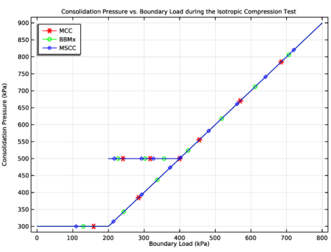
In the Settings window for 1D Plot Group, type Consolidation Pressure vs. Boundary Load in the Label text field.
3
Locate the Data section. From the Dataset list, choose Study: Test Material [Modified Cam-Clay Model]/Solution 1 (solidtm1sol1).
4
Locate the Title section. From the Title type list, choose Manual.
5
In the Title text area, type Consolidation Pressure vs. Boundary Load during the Isotropic Compression Test.
6
Locate the Plot Settings section.
7
Select the x-axis label check box. In the associated text field, type Boundary Load (kPa).
8
Select the y-axis label check box. In the associated text field, type Consolidation Pressure (kPa).
Point Graph 1
1
Right-click Consolidation Pressure vs. Boundary Load and choose Point Graph.
2
3
In the Settings window for Point Graph, click Replace Expression in the upper-right corner of the y-Axis Data section. From the menu, choose Component: Test Material [Modified Cam-Clay Model] (solidtm1comp)>Solid Mechanics>Soil material properties>Modified Cam-Clay>solid1.epsm1.pc - Consolidation pressure - Pa.
4
Locate the y-Axis Data section. From the Unit list, choose kPa.
5
Locate the x-Axis Data section. From the Parameter list, choose Expression.
6
In the Expression text field, type Pressure(para).
7
From the Unit list, choose kPa.
8
Locate the Coloring and Style section. From the Color list, choose Red.
9
Find the Line markers subsection. From the Marker list, choose Asterisk.
10
From the Positioning list, choose Interpolated.
11
Locate the Legends section. Select the Show legends check box.
12
From the Legends list, choose Manual.
13
Point Graph 2
1
In the Model Builder window, right-click Consolidation Pressure vs. Boundary Load and choose Point Graph.
2
In the Settings window for Point Graph, locate the Data section.
3
From the Dataset list, choose Study: Test Material [Extended Barcelona Basic Model]/Solution 1a (solidtm2sol1).
4
5
Click Replace Expression in the upper-right corner of the y-Axis Data section. From the menu, choose Component: Test Material [Extended Barcelona Basic Model] (solidtm2comp)>Solid Mechanics>Soil material properties>Extended Barcelona Basic>solid2.epsm2.pc - Consolidation pressure at saturation - Pa.
6
Locate the y-Axis Data section. From the Unit list, choose kPa.
7
Locate the x-Axis Data section. From the Parameter list, choose Expression.
8
In the Expression text field, type Pressure(para).
9
From the Unit list, choose kPa.
10
Locate the Coloring and Style section. From the Color list, choose Green.
11
Find the Line markers subsection. From the Marker list, choose Circle.
12
From the Positioning list, choose Interpolated.
13
In the Number text field, type 10.
14
Locate the Legends section. Select the Show legends check box.
15
From the Legends list, choose Manual.
16
Point Graph 3
1
Right-click Consolidation Pressure vs. Boundary Load and choose Point Graph.
2
In the Settings window for Point Graph, locate the Data section.
3
From the Dataset list, choose Study: Test Material [Modified Structured Cam-Clay Model]/Solution 1b (solidtm3sol1).
4
5
Click Replace Expression in the upper-right corner of the y-Axis Data section. From the menu, choose Component: Test Material [Modified Structured Cam-Clay Model] (solidtm3comp)>Solid Mechanics>Soil material properties>Modified Structured Cam-Clay>solid3.epsm3.pc - Consolidation pressure - Pa.
6
Locate the y-Axis Data section. From the Unit list, choose kPa.
7
Locate the x-Axis Data section. From the Parameter list, choose Expression.
8
In the Expression text field, type Pressure(para).
9
From the Unit list, choose kPa.
10
Locate the Coloring and Style section. From the Color list, choose Blue.
11
Find the Line markers subsection. From the Marker list, choose Diamond.
12
From the Positioning list, choose Interpolated.
13
In the Number text field, type 12.
14
Locate the Legends section. Select the Show legends check box.
15
From the Legends list, choose Manual.
16
Consolidation Pressure vs. Boundary Load
1
In the Model Builder window, click Consolidation Pressure vs. Boundary Load.
2
In the Settings window for 1D Plot Group, locate the Legend section.
3
From the Position list, choose Upper left.
4
In the Consolidation Pressure vs. Boundary Load toolbar, click  Plot.
Evaluate the void ratio at the final state for all three soil models.
Final Void Ratio
1
In the Results toolbar, click  Evaluation Group.
2
In the Settings window for Evaluation Group, type Final Void Ratio in the Label text field.
3
Locate the Data section. From the Dataset list, choose Study: Test Material [Modified Cam-Clay Model]/Solution 1 (solidtm1sol1).
4
From the Parameter selection (para) list, choose Last.
Point Evaluation 1
1
In the Final Void Ratio toolbar, click  Point Evaluation.
2
3
In the Settings window for Point Evaluation, click Replace Expression in the upper-right corner of the Expressions section. From the menu, choose Component: Test Material [Modified Cam-Clay Model] (solidtm1comp)>Solid Mechanics>Soil material properties>Modified Cam-Clay>solid1.epsm1.evoid - Void ratio.
4
Locate the Expressions section. In the table, enter the following settings:
Point Evaluation 2
1
Right-click Point Evaluation 1 and choose Duplicate.
2
In the Settings window for Point Evaluation, locate the Data section.
3
From the Dataset list, choose Study: Test Material [Extended Barcelona Basic Model]/Solution 1a (solidtm2sol1).
4
From the Parameter selection (para) list, choose Last.
5
6
Locate the Expressions section. In the table, enter the following settings:
Point Evaluation 3
1
Right-click Point Evaluation 2 and choose Duplicate.
2
In the Settings window for Point Evaluation, locate the Data section.
3
From the Dataset list, choose Study: Test Material [Modified Structured Cam-Clay Model]/Solution 1b (solidtm3sol1).
4
From the Parameter selection (para) list, choose Last.
5
6
Locate the Expressions section. In the table, enter the following settings:
Final Void Ratio
1
In the Model Builder window, click Final Void Ratio.
2
In the Settings window for Evaluation Group, click to expand the Format section.
3
From the Include parameters list, choose Off.
4
In the Final Void Ratio toolbar, click  Evaluate.