
|
|
|


|
1
|
|
2
|
In the Application Libraries window, select Fuel Cell and Electrolyzer Module>Fuel Cells>fuel_cell_cathode in the tree.
|
|
3
|
Click
|
|
1
|
|
2
|
|
1
|
|
2
|
|
1
|
|
2
|
In the Settings window for Volume, click Replace Expression in the upper-right corner of the Expression section. From the menu, choose Component 1 (comp1)>Hydrogen Fuel Cell>fc.RH - Relative humidity.
|
|
1
|
|
2
|
|
3
|
|
4
|
|
1
|
|
2
|
|
3
|
In the Settings window for Table, type Oversaturated, no liquid water transport in the Label text field.
|
|
1
|
|
2
|
|
3
|
In the tree, select Fluid Flow>Multiphase Flow>Phase Transport>Phase Transport in Porous Media (phtr).
|
|
4
|
Click to expand the Dependent Variables section. In the Volume fractions table, enter the following settings:
|
|
5
|
|
6
|
|
1
|
|
2
|
|
1
|
In the Model Builder window, under Component 1 (comp1) right-click Definitions and choose Variables.
|
|
2
|
|
3
|
|
4
|
Browse to the model’s Application Libraries folder and double-click the file fuel_cell_cathode_with_liquid_water_variables.txt.
|
|
1
|
|
2
|
|
3
|
|
4
|
Click
|
|
5
|
Browse to the model’s Application Libraries folder and double-click the file fuel_cell_cathode_with_liquid_water_pc.txt.
|
|
6
|
Click
|
|
7
|
|
8
|
|
9
|
|
10
|
In the Function table, enter the following settings:
|
|
11
|
|
12
|
|
13
|
|
1
|
In the Model Builder window, expand the Component 1 (comp1)>Hydrogen Fuel Cell (fc) node, then click Hydrogen Fuel Cell (fc).
|
|
2
|
|
3
|
|
1
|
|
2
|
In the Settings window for Water Condensation-Evaporation, locate the Condensation-Evaporation Rate section.
|
|
3
|
|
1
|
In the Model Builder window, under Component 1 (comp1)>Hydrogen Fuel Cell (fc) click O2 Gas Diffusion Electrode 1.
|
|
2
|
|
3
|
|
1
|
In the Model Builder window, under Component 1 (comp1) click Phase Transport in Porous Media (phtr).
|
|
2
|
|
3
|
|
1
|
In the Model Builder window, under Component 1 (comp1)>Phase Transport in Porous Media (phtr) click Phase and Porous Media Transport Properties 1.
|
|
2
|
In the Settings window for Phase and Porous Media Transport Properties, locate the Model Input section.
|
|
3
|
|
4
|
|
5
|
|
6
|
|
7
|
|
8
|
|
9
|
Locate the Matrix Properties section. From the εp list, choose User defined. In the associated text field, type eps_gas.
|
|
10
|
|
1
|
|
2
|
|
3
|
|
4
|
|
5
|
|
1
|
|
2
|
|
3
|
|
1
|
|
2
|
|
3
|
|
4
|
|
1
|
|
2
|
In the Settings window for Stationary, type Stationary - Excluding Phase Transport in the Label text field.
|
|
3
|
Locate the Physics and Variables Selection section. In the table, clear the Solve for check box for Phase Transport in Porous Media (phtr).
|
|
1
|
|
2
|
In the Settings window for Stationary, type Stationary - Phase Transport Only in the Label text field.
|
|
3
|
Locate the Physics and Variables Selection section. In the table, clear the Solve for check box for Hydrogen Fuel Cell (fc).
|
|
1
|
|
2
|
|
1
|
|
2
|
|
1
|
|
2
|
|
1
|
|
2
|
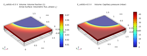
In the Settings window for Volume, click Replace Expression in the upper-right corner of the Expression section. From the menu, choose Component 1 (comp1)>Phase Transport in Porous Media>s_l - Volume fraction.
|
|
3
|
|
1
|
|
2
|
In the Settings window for Arrow Surface, click Replace Expression in the upper-right corner of the Expression section. From the menu, choose Component 1 (comp1)>Phase Transport in Porous Media>phtr.ux_s_l,...,phtr.uz_s_l - Volumetric flux, phase s_l.
|
|
3
|
|
4
|
|
1
|
|
3
|
|
1
|
|
2
|
|
1
|
|
2
|
In the Settings window for Volume, click Replace Expression in the upper-right corner of the Expression section. From the menu, choose Component 1 (comp1)>Definitions>Variables>pc - Capillary pressure - Pa.
|
|
3
|
|
4
|
|
1
|
In the Model Builder window, expand the Polarization Curve node, then click Probe Table Graph: Limited O2 gas phase transport.
|
|
2
|
|
1
|
|
2
|
|
3
|
|
4
|
Locate the Legends section. In the table, enter the following settings:
|
|
5
|


