PDF

High-Cycle Fatigue Analysis of a Cylindrical Test Specimen
Introduction
This is a benchmark model for the Fatigue Module. A cylindrical test specimen is subjected to nonproportional loading. Three stress based models — Findley, Matake, and Normal stress — are compared to analytical values and to each other. The nonsmooth behavior of the Matake model is captured and discussed.
Model Definition
A cylindrical test specimen with a geometry according to Figure 1 is subjected to fatigue testing. A combination of an axial force and a twisting moment is applied in such a way that the stress scenario shown in Figure 2 is affecting the central thin part of the specimen. The maximum shear stress is present at the outer radius of the bar.
Figure 1: Geometry of the test specimen.
Figure 2: Stress history at the outer radius in the central part of the specimen.
This stress state can be simulated with a cyclic normal force of 15708 N and a cyclic twisting moment of 22.672 Nm.
The specimen is made from mild steel with a Young’s modulus E of 210 GPa and a Poisson’s ratio ν of 0.3.
The examined fatigue criteria are Findley, Matake, and Normal stress. Material parameters are calculated from uniaxial fatigue tests. Results from two tests are available.
In the first test, the material is tested in reversed tension-compression, which means that the stress amplitude is alternating around zero stress, and the endurance limit is found to be  MPa.
In the second test, the material is tested in pure tension, where the stress is pulsating between zero to two times the stress amplitude. The endurance limit is then  MPa. The subscript of the endurance limit shows the R-value of the test.
Findley parameters are related to the fatigue test data via
and can thus be computed as fF = 213 MPa and kF = 0.20.
Matake parameters are related to the fatigue test data via
which gives fM = 223 MPa and kF = 0.27. In the Normal stress model, the stress limit equals twice the stress amplitude of the fatigue test. The model does not take into account the R-value dependency, and therefore two different limits are obtained. In order to give conservative results, the lower limit, ,is chosen and thus the model parameter is fN = 576 MPa. This actually indicates that normal stress may not be a good criterion for this material.
Results and Discussion
The load cycle is obtained in four load steps. The resulting stress at the outer radius of the thin section follows the specification, see Figure 3.
Figure 3: Resulting stresses at the outer radius of the smallest section of the specimen.
The three fatigue criteria evaluated on the boundary of the specimen are presented in Figure 4, Figure 5, and Figure 6.
In this example, it is the central part of the specimen which is in focus for the evaluation, even though the maximum fatigue usage is slightly higher in the fillets.
The Findley model shows that the highest fatigue usage factor is found at the transition between the thin cylinder and the fillet, with the value being 0.99 against 0.95 in the center. A smooth transition in the results indicates that the specified search resolution for the critical plane is sufficient to correctly capture the fatigue response.
Figure 4: Fatigue usage factor Findley criterion.
The Matake criterion gives less smooth results. The reason can be found in the definition of the criterion, which selects the critical plane using the shear stresses only and then adds the normal stress. This is discussed in more detail on page 10. The analysis of the test specimen predicts a fatigue usage factor in the range from 0.79 to 0.99 in the central part, as compared to 1.03 at some points at the transition from the thin cylinder to the notch.
Figure 5: Fatigue usage factor Matake criterion.
The Normal Stress criterion predicts yet another fatigue usage factor. Again, the highest fatigue usage factor is found on the transition from the thin section to the notch, 0.93, as compared to the center of the specimen, where it is 0.88.
Figure 6: Fatigue usage factor Normal stress criterion.
The stress state on the surface in the central part of the specimen can be evaluated using analytical expressions. As there are no tractions on the boundary, it is in a state of plane stress. Therefore, the search for the critical plane can be reduced to two dimensions. In that case, the normal and shear stresses on a plane can be obtained as
(1)
where σa and σb are orthogonal normal stresses, and τab is the shear stress. The orientation angle is calculated from the axis of σa toward σb. In the current example, the σa is the axial stress, and τab as the shear stress caused by the twisting moment.
In the current example, a search resolution of Q = 11 is used. This gives a 9° angular increment in the critical plane evaluation. Using Equation 1, the normal and shear stresses evaluated on discrete planes are given in Table 1 and Table 2. The number in the subscripts indicates the load case.
(°)
σn,1(MPa)
σn,2(MPa)
σn,3(MPa)
σn,4(MPa)
σn,max(MPa)
Δσn(MPa)
 
(°)
τ1 (MPa)
τ2 (MPa)
τ3 (MPa)
τ4 (MPa)
Δτ (MPa)
The Findley criterion searches for a critical plane where a combination between the shear stress range and the normal stress is highest. This stress is shown in the second column of Table 3, where it can be seen that 202 MPa is found at planes oriented at 18° and 162°. This results into a usage factor of 202/213 = 0.95, which is in good agreement with the computed results.
(°)
Δσn(MPa)
The Matake criterion selects the critical plane as the one with the largest shear stress range. This occurs at orientations 18°, 72°, 108°, and 162° where the range is 304 MPa, see Table 2. The maximum normal stress on those planes is either 87 MPa or 249 MPa, see Table 1 and the Matake stress is either 219 MPa or 175 MPa, see Table 3. Since the Matake criterion does not contain the normal stress in the selection of the critical plane, the fatigue criteria is calculated with either one of them. In Figure 5, this feature is demonstrated by the nonsmooth results. The analytical values at the critical planes for the Matake usage factor are 219/223 = 0.98 and 175/223 = 0.78, which is in good agreement with the computed results.
The Normal stress criterion considers the plane with the largest normal stress range. The last column of Table 3 shows that this is found on planes with orientations 27° and 153° where the range is 504 MPa. This results into a fatigue usage factor of 504/576 = 0.88, which is in good agreement with the computed results.
Notes About the COMSOL Implementation
In the critical plane evaluation, a search resolution Q indicates the number of evaluation point along 90° of a unit circle. The angle between two evaluation points is then at most (90°)/(Q1).
Application Library path: Fatigue_Module/Verification_Examples/cylindrical_test_specimen
Modeling Instructions
From the File menu, choose New.
New
In the New window, click  Model Wizard.
Model Wizard
1
In the Model Wizard window, click  3D.
2
In the Select Physics tree, select Structural Mechanics>Solid Mechanics (solid).
3
Click Add.
4
Click  Study.
5
In the Select Study tree, select General Studies>Stationary.
6
Geometry 1
1
In the Model Builder window, under Component 1 (comp1) click Geometry 1.
2
In the Settings window for Geometry, locate the Units section.
3
From the Length unit list, choose mm.
Global Definitions
Parameters 1
1
In the Model Builder window, under Global Definitions click Parameters 1.
2
In the Settings window for Parameters, locate the Parameters section.
3
Geometry 1
Work Plane 1 (wp1)
1
In the Geometry toolbar, click  Work Plane.
2
In the Settings window for Work Plane, click  Show Work Plane.
Work Plane 1 (wp1)>Plane Geometry
In the Model Builder window, click Plane Geometry.
Work Plane 1 (wp1)>Polygon 1 (pol1)
1
In the Work Plane toolbar, click  Polygon.
2
In the Settings window for Polygon, locate the Object Type section.
3
From the Type list, choose Open curve.
4
Locate the Coordinates section. From the Data source list, choose Vectors.
5
In the xw text field, type 5 5 0 0 10 10 6.01.
6
In the yw text field, type 20 0 0 50 50 30 30.
7
Click the  Zoom Extents button in the Graphics toolbar.
Work Plane 1 (wp1)>Quadratic Bézier 1 (qb1)
1
In the Work Plane toolbar, click  More Primitives and choose Quadratic Bézier.
2
In the Settings window for Quadratic Bézier, locate the Control Points section.
3
In row 1, set xw to 6.01.
4
In row 2, set xw to 5.25.
5
In row 3, set xw to 5.
6
In row 1, set yw to 30.
7
In row 2, set yw to 25.
8
In row 3, set yw to 20.
Work Plane 1 (wp1)>Convert to Solid 1 (csol1)
1
In the Work Plane toolbar, click  Conversions and choose Convert to Solid.
2
Click in the Graphics window and then press Ctrl+A to select both objects.
3
In the Settings window for Convert to Solid, click  Build Selected.
Work Plane 1 (wp1)>Fillet 1 (fil1)
1
In the Work Plane toolbar, click  Fillet.
2
On the object csol1, select Point 5 only.
3
In the Settings window for Fillet, locate the Radius section.
4
In the Radius text field, type 4.
Work Plane 1 (wp1)>Mirror 1 (mir1)
1
In the Work Plane toolbar, click  Transforms and choose Mirror.
2
3
In the Settings window for Mirror, locate the Normal Vector to Line of Reflection section.
4
In the xw text field, type 0.
5
In the yw text field, type 1.
6
Locate the Input section. Select the Keep input objects check box.
7
Click  Build Selected.
8
Click the  Zoom Extents button in the Graphics toolbar.
Work Plane 1 (wp1)>Union 1 (uni1)
1
In the Work Plane toolbar, click  Booleans and Partitions and choose Union.
2
Click in the Graphics window and then press Ctrl+A to select both objects.
3
In the Settings window for Union, locate the Union section.
4
Clear the Keep interior boundaries check box.
5
In the Work Plane toolbar, click  Build All.
Revolve 1 (rev1)
1
In the Model Builder window, under Component 1 (comp1)>Geometry 1 right-click Work Plane 1 (wp1) and choose Revolve.
2
In the Settings window for Revolve, locate the Revolution Angles section.
3
Clear the Keep original faces check box.
4
Click  Build All Objects.
5
Click the  Zoom Extents button in the Graphics toolbar.
Materials
Material 1 (mat1)
1
In the Model Builder window, under Component 1 (comp1) right-click Materials and choose Blank Material.
2
In the Settings window for Material, locate the Material Contents section.
3
Solid Mechanics (solid)
Fixed Constraint 1
1
In the Model Builder window, under Component 1 (comp1) right-click Solid Mechanics (solid) and choose Fixed Constraint.
2
Rigid Connector 1
1
In the Physics toolbar, click  Boundaries and choose Rigid Connector.
2
Applied Force 1
1
In the Physics toolbar, click  Attributes and choose Applied Force.
2
In the Settings window for Applied Force, locate the Applied Force section.
3
Specify the F vector as
4
In the Physics toolbar, click  Load Group and choose New Load Group.
Rigid Connector 1
In the Model Builder window, click Rigid Connector 1.
Applied Moment 1
1
In the Physics toolbar, click  Attributes and choose Applied Moment.
2
In the Settings window for Applied Moment, locate the Applied Moment section.
3
Specify the M vector as
4
In the Physics toolbar, click  Load Group and choose New Load Group.
Global Definitions
Load Group: Force
1
In the Model Builder window, under Global Definitions>Load and Constraint Groups click Load Group 1.
2
In the Settings window for Load Group, type Load Group: Force in the Label text field.
3
In the Parameter name text field, type lgF.
Load Group: Moment
1
In the Model Builder window, under Global Definitions>Load and Constraint Groups click Load Group 2.
2
In the Settings window for Load Group, type Load Group: Moment in the Label text field.
3
In the Parameter name text field, type lgM.
Create a load cycle consisting of four load cases.
Study 1
Step 1: Stationary
1
In the Model Builder window, under Study 1 click Step 1: Stationary.
2
In the Settings window for Stationary, click to expand the Study Extensions section.
3
Select the Define load cases check box.
4
Click Add four times.
5
6
In the Home toolbar, click  Compute.
Results
Verify stresses at the center of the test specimen.
Stresses
1
In the Home toolbar, click  Add Plot Group and choose 1D Plot Group.
2
In the Settings window for 1D Plot Group, type Stresses in the Label text field.
Point Graph 1
1
Right-click Stresses and choose Point Graph.
2
It might be easier to select the correct point by using the Selection List window. To open this window, in the Home toolbar click Windows and choose Selection List. (If you are running the cross-platform desktop, you find Windows in the main menu.)
3
In the Settings window for Point Graph, click Replace Expression in the upper-right corner of the y-Axis Data section. From the menu, choose Component 1 (comp1)>Solid Mechanics>Stress (Gauss points)>Second Piola-Kirchhoff stress, Gauss point evaluation (material and geometry frames) - N/m²>solid.SGpYY - Second Piola-Kirchhoff stress, Gauss point evaluation, YY-component.
4
Locate the y-Axis Data section. From the Unit list, choose MPa.
5
Click to expand the Legends section. Select the Show legends check box.
6
From the Legends list, choose Manual.
7
Point Graph 2
1
Right-click Point Graph 1 and choose Duplicate.
2
In the Settings window for Point Graph, locate the y-Axis Data section.
3
In the Expression text field, type solid.SGpXY.
4
Locate the Legends section. In the table, enter the following settings:
Point Graph 3
1
Right-click Point Graph 2 and choose Duplicate.
2
In the Settings window for Point Graph, locate the y-Axis Data section.
3
In the Expression text field, type solid.misesGp.
4
Locate the Legends section. In the table, enter the following settings:
Stresses
1
In the Model Builder window, click Stresses.
2
In the Settings window for 1D Plot Group, click to expand the Title section.
3
From the Title type list, choose None.
4
Locate the Plot Settings section.
5
Select the y-axis label check box. In the associated text field, type Stress (MPa).
6
In the Stresses toolbar, click  Plot.
Add Physics
1
In the Home toolbar, click  Add Physics to open the Add Physics window.
2
Go to the Add Physics window.
3
In the tree, select Structural Mechanics>Fatigue (ftg).
4
Find the Physics interfaces in study subsection. In the table, clear the Solve check box for Study 1.
5
Click Add to Component 1 in the window toolbar.
Fatigue Findley
In the Settings window for Fatigue, type Fatigue Findley in the Label text field.
Stress-Based 1
1
Right-click Component 1 (comp1)>Fatigue Findley and choose the boundary evaluation Stress-Based.
2
In the Settings window for Stress-Based, locate the Boundary Selection section.
3
From the Selection list, choose All boundaries.
4
Locate the Solution Field section. From the Physics interface list, choose Solid Mechanics (solid).
Add Physics
1
Go to the Add Physics window.
2
In the tree, select Structural Mechanics>Fatigue (ftg).
3
Find the Physics interfaces in study subsection. In the table, clear the Solve check box for Study 1.
4
Click Add to Component 1 in the window toolbar.
Fatigue Matake
1
In the Settings window for Fatigue, type Fatigue Matake in the Label text field.
2
Right-click Component 1 (comp1)>Fatigue Matake and choose the boundary evaluation Stress-Based.
Stress-Based 1
1
In the Settings window for Stress-Based, locate the Boundary Selection section.
2
From the Selection list, choose All boundaries.
3
Locate the Fatigue Model Selection section. From the Criterion list, choose Matake.
4
Locate the Solution Field section. From the Physics interface list, choose Solid Mechanics (solid).
Add Physics
1
Go to the Add Physics window.
2
In the tree, select Structural Mechanics>Fatigue (ftg).
3
Find the Physics interfaces in study subsection. In the table, clear the Solve check box for Study 1.
4
Click Add to Component 1 in the window toolbar.
5
In the Physics toolbar, click  Add Physics to close the Add Physics window.
Fatigue Normal Stress
1
In the Settings window for Fatigue, type Fatigue Normal Stress in the Label text field.
2
Right-click Component 1 (comp1)>Fatigue Normal Stress and choose the boundary evaluation Stress-Based.
Stress-Based 1
1
In the Settings window for Stress-Based, locate the Boundary Selection section.
2
From the Selection list, choose All boundaries.
3
Locate the Fatigue Model Selection section. From the Criterion list, choose Normal stress.
4
Locate the Solution Field section. From the Physics interface list, choose Solid Mechanics (solid).
Materials
Material 2 (mat2)
1
In the Model Builder window, under Component 1 (comp1) right-click Materials and choose Blank Material.
2
In the Settings window for Material, locate the Geometric Entity Selection section.
3
From the Geometric entity level list, choose Boundary.
4
From the Selection list, choose All boundaries.
5
Locate the Material Contents section. In the table, enter the following settings:
Add Study
1
In the Home toolbar, click  Add Study to open the Add Study window.
2
Go to the Add Study window.
3
Find the Physics interfaces in study subsection. In the table, clear the Solve check box for Solid Mechanics (solid).
4
Find the Studies subsection. In the Select Study tree, select Preset Studies for Selected Physics Interfaces>Fatigue.
5
Click Add Study in the window toolbar.
6
In the Home toolbar, click  Add Study to close the Add Study window.
Study 2
Step 1: Fatigue
1
In the Settings window for Fatigue, locate the Values of Dependent Variables section.
2
Find the Values of variables not solved for subsection. From the Settings list, choose User controlled.
3
From the Method list, choose Solution.
4
From the Study list, choose Study 1, Stationary.
5
In the Home toolbar, click  Compute.
Results
Fatigue Usage Factor (Findley)
In the Settings window for 3D Plot Group, type Fatigue Usage Factor (Findley) in the Label text field.
Fatigue Usage Factor (Matake)
1
In the Model Builder window, under Results click Fatigue Usage Factor (ftg2).
2
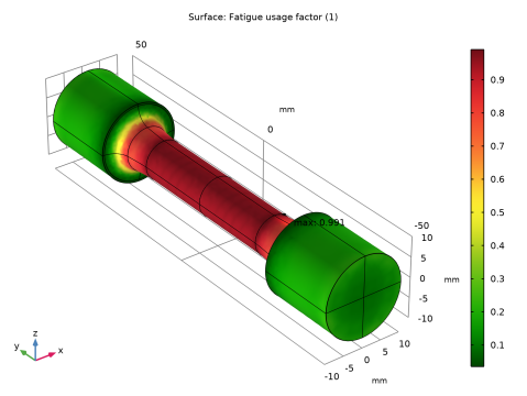
In the Settings window for 3D Plot Group, type Fatigue Usage Factor (Matake) in the Label text field.
Fatigue Usage Factor (Normal Stress)
1
In the Model Builder window, under Results click Fatigue Usage Factor (ftg3).
2
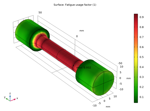
In the Settings window for 3D Plot Group, type Fatigue Usage Factor (Normal Stress) in the Label text field.