PDF

Cycle Counting in Fatigue Analysis — Benchmark
Introduction
In this benchmark model for the Rainflow counting algorithm, values computed by the Fatigue Module in COMSOL are compared with the ASTM standard E1049-85 (Ref. 1). An extension to the benchmark compares the Palmgren-Miner cumulative damage model to analytical expressions.
Model Definition
A flat test specimen is subjected to a repeated load cycle. The material has elastic properties defined by Young’s modulus E = 69 GPa and Poisson’s ratio ν = 0.34. The thickness of the specimen is 6.25 mm. The remaining dimensions are given in Figure 1.
Figure 1: Flat test specimen. Dimensions are given in mm.
The Wöhler diagram (S-N curve) is given by the expression
where σa is the stress amplitude, R is the R-value and N is the number of cycles to failure for a constant stress cycle defined by σa and R. The relation is valid for , while the parameter is seen as infinite life and it should not be taken into account in damage calculations.
An ASTM cycle (Ref. 1) is evaluated in the example. The load history of the cycle is presented in Table 1.
The unit load can be chosen arbitrarily and is here selected so that one unit load corresponds to 10 MPa stress in the central cross section.
The ASTM example is further extended to examine the fatigue damage caused by 100000 blocks of the cycle.
In the test specimen, the stress state in the central part away from the fillets does not vary with the position. Therefore, any point in the central thin cross section can be chosen for evaluation.
Results and Discussion
Because of the symmetry, only a quarter of the test specimen is modeled. The 2D Solid Mechanics interface is used with a plane stress assumption. Figure 2 shows the axial stress caused by a unit load. Although a quarter of the specimen was modeled, the results for the whole specimen can be examined using datasets of the type Mirror 2D.
Figure 2: Axial stress in the specimen caused by a unit load.
The Cumulative Damage feature generates results of the cycle counting algorithm as well as a damage calculation. A point in the thin central cross section is evaluated. The applied load cycle, see Table 1, is quantified with the Rainflow Counting algorithm and shown in Figure 3. The ASTM results (Ref. 1) are shown in Table 2
σa (MPa)
σm (MPa)
here, σm is the cycle mean stress amplitude and n is number of cycles.
Figure 3: Load cycle quantified with the Rainflow Counting option.
The Rainflow Counting results by ASTM and COMSOL are in perfect agreement.
The evaluation of the cumulative damage is now compared against analytical expressions. In the Palmgren-Miner model, the damage is calculated for each stress bin. The number of cycles to failure for a constant cycle is taken from the S-N curve which is evaluated at the center of the bin.
With the chosen bin discretization the damage is evaluated at following bin stress centers:
 = 17.1 MPa, 21.4 MPa, 25.7 MPa, 30.0 MPa, 34.3 MPa, 38.6 MPa, 42.9 MPa
and
 = -8.0 MPa, -4.0 MPa, 0.0 MPa, 4.0 MPa, 8.0 MPa
The key values for the damaging bins are presented in Table 3. The superscript ‘b’ denotes that the variable is evaluated at the bin center.
σa (MPa)
σm (MPa)
σab (MPa)
σmb (MPa)
Rb
nb
Nb
The fatigue usage factor fus following the Palmgren-Miner linear damage rule is calculated using the expression
(1)
where m is the number or repeatable block and p is the number of bins.
Following Equation 1 the fatigue usage factor of the ASTM cycles is . The COMSOL result is fus= 0.182. The small discrepancy between the results is attributed to the evaluation of the S-N curve.
The relative damage contribution from each bin is shown in Figure 4.
Figure 4: Contribution of each stress bin to the fatigue usage.
The Cumulative Damage model is based on the Palmgren-Miner linear damage rule. It is a discrete model in the sense that the calculations are based on stress bins which hold all stress cycles within a certain stress amplitude and mean stress range.
In this example, the stress amplitude range in a bin is 20 MPa/5=4 MPa and the mean stress range in a bin is 30 MPa/7 MPa = 4.3 MPa. By changing the bin discretization, the graph showing counted stress cycles in Figure 3, appears with a different resolution.
As for the results of the relative damage in Figure 4, a change in discretization can affect the results significantly. The damage is evaluated based on the bin stresses and not true cycle stresses. Consider the cycle defined by σa = 45.0 MPa and σm = 5.0 MPa. It is evaluated in a bin defined by  = 42.9 MPa and  = 4.0 MPa. Since bin stresses are lower than true stresses in that cycle, they predict less damage and thus give a nonconservative contribution to the fatigue usage factor.
Notes About the COMSOL Implementation
In the Cumulative Damaged feature, you can use three different types of S-N curves — S-N curve with R-value dependence, S-N curve with mean stress dependence, or S-N curve for amplitude stress. In this model, the S-N curve is defined using the R-value definition. The arguments to this S-N curve are specified by first giving the R-value followed by the number of cycles, as it is done in the Analytic function in the Arguments field.
Reference
1. ASTM International, Standard Practices for Cycle Counting in Fatigue Analysis, Designation: E1049-85 (Reapproved 2011).
Application Library path: Fatigue_Module/Verification_Examples/cycle_counting_benchmark
Modeling Instructions
From the File menu, choose New.
New
In the New window, click  Model Wizard.
Model Wizard
1
In the Model Wizard window, click  2D.
2
In the Select Physics tree, select Structural Mechanics>Solid Mechanics (solid).
3
Click Add.
4
Click  Study.
5
In the Select Study tree, select General Studies>Stationary.
6
Geometry 1
1
In the Model Builder window, under Component 1 (comp1) click Geometry 1.
2
In the Settings window for Geometry, locate the Units section.
3
From the Length unit list, choose mm.
Rectangle 1 (r1)
1
In the Geometry toolbar, click  Rectangle.
2
In the Settings window for Rectangle, locate the Size and Shape section.
3
In the Width text field, type 10.
4
In the Height text field, type 100.
Rectangle 2 (r2)
1
In the Geometry toolbar, click  Rectangle.
2
In the Settings window for Rectangle, locate the Size and Shape section.
3
In the Width text field, type 10-6.25.
4
In the Height text field, type 50-sqrt(12.5^2-8.75^2).
5
Locate the Position section. In the x text field, type 6.25.
Circle 1 (c1)
1
In the Geometry toolbar, click  Circle.
2
In the Settings window for Circle, locate the Position section.
3
In the x text field, type 6.25+12.5.
4
In the y text field, type 50-sqrt(12.5^2-8.75^2).
5
Locate the Size and Shape section. In the Radius text field, type 12.5.
Difference 1 (dif1)
1
In the Geometry toolbar, click  Booleans and Partitions and choose Difference.
2
Global Definitions
Specify the load cycle.
Interpolation 1 (int1)
1
In the Home toolbar, click  Functions and choose Global>Interpolation.
2
In the Settings window for Interpolation, locate the Definition section.
3
Solid Mechanics (solid)
1
In the Model Builder window, under Component 1 (comp1) click Solid Mechanics (solid).
2
In the Settings window for Solid Mechanics, locate the 2D Approximation section.
3
4
Locate the Thickness section. In the d text field, type 0.00625.
Symmetry 1
1
In the Physics toolbar, click  Boundaries and choose Symmetry.
2
Boundary Load 1
1
In the Physics toolbar, click  Boundaries and choose Boundary Load.
2
3
In the Settings window for Boundary Load, locate the Force section.
4
From the Load type list, choose Total force.
5
Specify the Ftot vector as
Global Definitions
Parameters 1
1
In the Model Builder window, under Global Definitions click Parameters 1.
2
In the Settings window for Parameters, locate the Parameters section.
3
Materials
Material 1 (mat1)
1
In the Model Builder window, under Component 1 (comp1) right-click Materials and choose Blank Material.
2
In the Settings window for Material, locate the Material Contents section.
3
Study 1
Step 1: Stationary
1
In the Model Builder window, under Study 1 click Step 1: Stationary.
2
In the Settings window for Stationary, click to expand the Study Extensions section.
3
Select the Auxiliary sweep check box.
4
5
6
In the Home toolbar, click  Compute.
Results
Stress (solid)
Mirror solution of a quarter of a specimen and create results for a full specimen.
Mirror 2D 1
1
In the Results toolbar, click  More Datasets and choose Mirror 2D.
2
In the Settings window for Mirror 2D, locate the Axis Data section.
3
In row Point 2, set Y to 100.
Mirror 2D 2
1
In the Results toolbar, click  More Datasets and choose Mirror 2D.
2
In the Settings window for Mirror 2D, locate the Data section.
3
From the Dataset list, choose Mirror 2D 1.
4
Locate the Axis Data section. In row Point 1, set x to -6.25.
5
In row Point 2, set x to 6.25 and y to 0.
Display stress state in the whole specimen.
Stress (solid)
1
In the Model Builder window, under Results click Stress (solid).
2
In the Settings window for 2D Plot Group, locate the Data section.
3
From the Dataset list, choose Mirror 2D 2.
4
From the Parameter value (case) list, choose 2.
5
Click to expand the Title section. From the Title type list, choose None.
6
Locate the Color Legend section. Select the Show units check box.
Surface 1
1
In the Model Builder window, expand the Stress (solid) node, then click Surface 1.
2
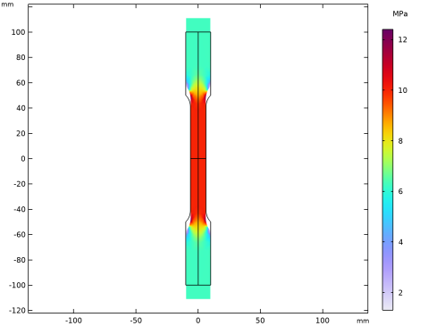
In the Settings window for Surface, click Replace Expression in the upper-right corner of the Expression section. From the menu, choose Component 1 (comp1)>Solid Mechanics>Stress (Gauss points)>Second Piola-Kirchhoff stress, Gauss point evaluation (material and geometry frames) - N/m²>solid.SGpYY - Second Piola-Kirchhoff stress, Gauss point evaluation, YY-component.
3
Locate the Expression section. From the Unit list, choose MPa.
4
In the Stress (solid) toolbar, click  Plot.
Load Cycle Response
1
In the Home toolbar, click  Add Plot Group and choose 1D Plot Group.
2
In the Settings window for 1D Plot Group, type Load Cycle Response in the Label text field.
Point Graph 1
1
Right-click Load Cycle Response and choose Point Graph.
2
3
In the Settings window for Point Graph, click Replace Expression in the upper-right corner of the y-Axis Data section. From the menu, choose Component 1 (comp1)>Solid Mechanics>Stress (Gauss points)>Second Piola-Kirchhoff stress, Gauss point evaluation (material and geometry frames) - N/m²>solid.SGpYY - Second Piola-Kirchhoff stress, Gauss point evaluation, YY-component.
4
Locate the y-Axis Data section. From the Unit list, choose MPa.
5
In the Load Cycle Response toolbar, click  Plot.
Global Definitions
Specify the load cycle.
Analytic 1 (an1)
1
In the Home toolbar, click  Functions and choose Global>Analytic.
2
In the Settings window for Analytic, locate the Definition section.
3
In the Arguments text field, type R, N.
4
In the Expression text field, type (94e6*(R/-0.36)^1.15)*N^-0.119.
Add Physics
1
In the Home toolbar, click  Add Physics to open the Add Physics window.
2
Go to the Add Physics window.
3
In the tree, select Structural Mechanics>Fatigue (ftg).
4
Find the Physics interfaces in study subsection. In the table, clear the Solve check box for Study 1.
5
Click Add to Component 1 in the window toolbar.
6
In the Home toolbar, click  Add Physics to close the Add Physics window.
Fatigue (ftg)
Cumulative Damage 1
1
Right-click Component 1 (comp1)>Fatigue (ftg) and choose the point evaluation Cumulative Damage.
Any point in the thin section away from the notch will give the same fatigue response.
2
3
In the Settings window for Cumulative Damage, locate the Solution Field section.
4
From the Physics interface list, choose Solid Mechanics (solid).
5
Locate the Cycle Counting Parameters section. Find the Discretization subsection. In the Nm text field, type 5.
6
In the Nr text field, type 7.
7
Locate the Damage Model Parameters section. From the fSN(R,N) list, choose an1.
8
In the m text field, type 100000.
Set cutoff which can be seen as a limit for infinite life that does not contribute to the damage.
9
Find the Evaluation settings subsection. In the Ncut text field, type 1e8.
Add Study
1
In the Home toolbar, click  Add Study to open the Add Study window.
2
Go to the Add Study window.
3
Find the Physics interfaces in study subsection. In the table, clear the Solve check box for Solid Mechanics (solid).
4
Find the Studies subsection. In the Select Study tree, select Preset Studies for Selected Physics Interfaces>Fatigue.
5
Click Add Study in the window toolbar.
6
In the Home toolbar, click  Add Study to close the Add Study window.
Study 2
Step 1: Fatigue
1
In the Settings window for Fatigue, locate the Values of Dependent Variables section.
2
Find the Values of variables not solved for subsection. From the Settings list, choose User controlled.
3
From the Method list, choose Solution.
4
From the Study list, choose Study 1, Stationary.
5
In the Home toolbar, click  Compute.
Results
Matrix Histogram 1
1
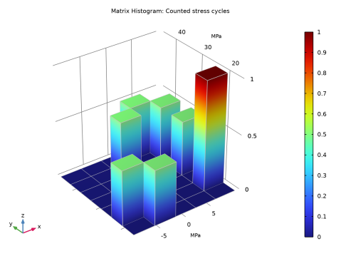
In the Model Builder window, expand the Stress Cycle Distribution (ftg) node, then click Matrix Histogram 1.
2
In the Settings window for Matrix Histogram, locate the Axes section.
3
From the Unit list, choose MPa.
4
In the Stress Cycle Distribution (ftg) toolbar, click  Plot.
5
Click the  Zoom Extents button in the Graphics toolbar.
Matrix Histogram 1
1
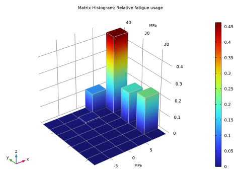
In the Model Builder window, expand the Fatigue Usage Distribution (ftg) node, then click Matrix Histogram 1.
2
In the Settings window for Matrix Histogram, locate the Axes section.
3
From the Unit list, choose MPa.
4
In the Fatigue Usage Distribution (ftg) toolbar, click  Plot.
5
Click the  Zoom Extents button in the Graphics toolbar.