|
|
|


 .
. 
|
1
|
|
2
|
In the Select Physics tree, select Electrochemistry>Primary and Secondary Current Distribution>Primary Current Distribution (cd).
|
|
3
|
Click Add.
|
|
4
|
Click
|
|
5
|
|
6
|
Click
|
|
1
|
|
2
|
|
3
|
|
4
|
Browse to the model’s Application Libraries folder and double-click the file rotating_cylinder_hull_cell_parameters.txt.
|
|
1
|
|
2
|
|
3
|
|
4
|
Browse to the model’s Application Libraries folder and double-click the file rotating_cylinder_hull_cell_polygon.txt.
|
|
5
|
|
1
|
|
2
|
|
3
|
|
4
|
|
5
|
|
6
|
|
7
|
Locate the Selections of Resulting Entities section. Select the Resulting objects selection check box.
|
|
8
|
|
9
|
|
1
|
|
2
|
|
3
|
|
4
|
Browse to the model’s Application Libraries folder and double-click the file rotating_cylinder_hull_cell_variables.txt.
|
|
1
|
|
2
|
|
3
|
|
5
|
|
1
|
|
2
|
|
3
|
|
5
|
|
1
|
In the Model Builder window, under Component 1 (comp1)>Primary Current Distribution (cd) click Electrolyte 1.
|
|
2
|
|
3
|
|
1
|
|
2
|
|
3
|
|
1
|
|
2
|
|
3
|
|
4
|
Locate the Electrode Phase Potential Condition section. From the Electrode phase potential condition list, choose Average current density.
|
|
5
|
|
1
|
|
2
|
|
3
|
|
4
|
|
1
|
|
1
|
|
3
|
|
4
|
|
5
|
|
6
|
|
1
|
|
2
|
|
1
|
|
1
|
|
2
|
|
1
|
|
2
|
|
3
|
Click OK.
|
|
1
|
|
2
|
|
3
|
|
1
|
|
2
|
|
3
|
|
4
|
|
5
|
|
6
|
In the Unit field, type .
|
|
7
|
|
8
|
|
9
|
Select the Description check box. In the associated text field, type Distance along the working electrode.
|
|
10
|
|
11
|
|
13
|
|
1
|
|
2
|
|
3
|
|
4
|
|
5
|
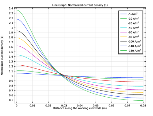
Locate the Legends section. In the table, enter the following settings:
|
|
6
|
|
1
|
|
2
|
In the Rename 1D Plot Group dialog box, type Normalized current density, Primary in the New label text field.
|
|
3
|
Click OK.
|
|
1
|
|
2
|
In the Settings window for Primary Current Distribution, locate the Current Distribution Type section.
|
|
3
|
|
1
|
In the Model Builder window, under Component 1 (comp1)>Secondary Current Distribution (cd)>Electrode Surface 1 click Electrode Reaction 1.
|
|
2
|
|
3
|
|
4
|
|
5
|
|
1
|
|
2
|
|
3
|
|
4
|
Click
|
|
6
|
|
1
|
|
2
|
|
3
|
Click OK.
|
|
1
|
|
2
|
|
3
|
|
1
|
|
2
|
|
3
|
|
4
|
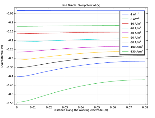
Click Replace Expression in the upper-right corner of the y-Axis Data section. From the menu, choose Component 1 (comp1)>Secondary Current Distribution>Electrode kinetics>cd.eta_er1 - Overpotential - V.
|
|
5
|
|
6
|
|
7
|
|
8
|
Select the Description check box. In the associated text field, type Distance along the working electrode.
|
|
9
|
|
10
|
|
1
|
|
2
|
|
1
|
|
2
|
|
3
|
|
4
|
|
5
|
|
1
|
|
2
|
In the Rename 1D Plot Group dialog box, type Normalized current density, Secondary in the New label text field.
|
|
3
|
Click OK.
|
|
1
|
|
2
|
|
3
|
|
4
|
|
5
|
|
1
|
|
2
|
|
3
|
|
1
|
In the Model Builder window, under Component 1 (comp1)>Transport of Diluted Species (tds) click Transport Properties 1.
|
|
2
|
|
3
|
|
1
|
|
2
|
|
3
|
|
1
|
|
3
|
|
4
|
|
5
|
|
1
|
|
2
|
|
3
|
|
1
|
In the Model Builder window, expand the Electrode Surface Coupling 1 node, then click Reaction Coefficients 1.
|
|
2
|
|
3
|
|
4
|
|
5
|
|
1
|
In the Model Builder window, under Component 1 (comp1)>Secondary Current Distribution (cd)>Electrode Surface 1 click Electrode Reaction 1.
|
|
2
|
|
3
|
|
1
|
|
2
|
|
4
|
|
1
|
|
2
|
|
3
|
|
4
|
Click Replace Expression in the upper-right corner of the y-Axis Data section. From the menu, choose Component 1 (comp1)>Secondary Current Distribution>Electrode kinetics>cd.eta_er1 - Overpotential - V.
|
|
5
|
|
6
|
|
7
|
|
8
|
Select the Description check box. In the associated text field, type Distance along the working electrode.
|
|
9
|
|
10
|
|
1
|
|
2
|
|
1
|
|
2
|
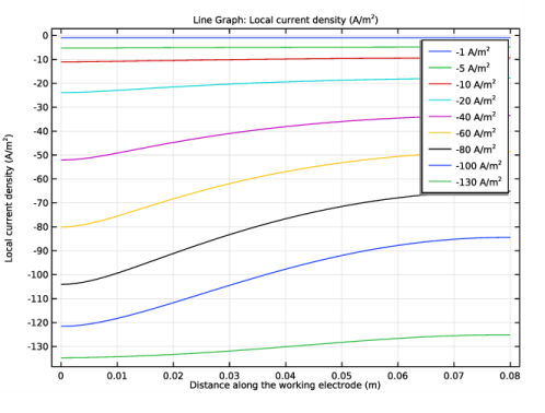
In the Settings window for Line Graph, click Replace Expression in the upper-right corner of the y-Axis Data section. From the menu, choose Component 1 (comp1)>Secondary Current Distribution>Electrode kinetics>cd.iloc_er1 - Local current density - A/m².
|
|
3
|
|
4
|
|
1
|
|
2
|
In the Settings window for 1D Plot Group, type Local current density, Tertiary in the Label text field.
|
|
1
|
In the Model Builder window, expand the Local current density, Tertiary 1 node, then click Line Graph 1.
|
|
2
|
|
3
|
|
4
|
|
5
|
|
1
|
|
2
|
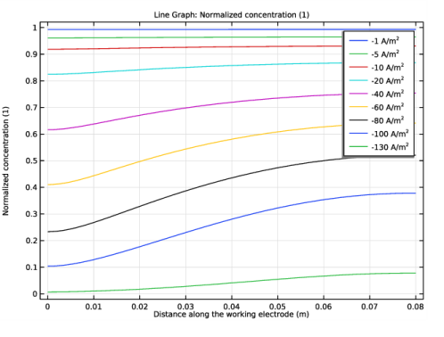
In the Rename 1D Plot Group dialog box, type Normalized concentration, Tertiary in the New label text field.
|
|
3
|
Click OK.
|
|
1
|
|
2
|
|
3
|
|
1
|
|
2
|
|
3
|
|
4
|
|
5
|
|
6
|
|
7
|
|
8
|
|
9
|
Select the Description check box. In the associated text field, type Distance along the working electrode.
|
|
10
|
|
11
|
|
13
|
|
1
|
|
2
|
|
3
|
|
4
|
|
5
|
|
6
|
|
7
|
Locate the Legends section. In the table, enter the following settings:
|
|
8
|
|
1
|
|
2
|
|
3
|
|
4
|
|
5
|
Locate the Legends section. In the table, enter the following settings:
|
|
6
|
|
1
|
|
2
|
In the Rename 1D Plot Group dialog box, type Current density comparison in the New label text field.
|
|
3
|
Click OK.
|