PDF

Corrosion Protection of a Ship Hull
Introduction
Impressed current cathodic protection (ICCP) is a commonly employed strategy to mitigate ship hull corrosion, by which an external current is applied to the hull surface, polarizing it to a lower potential. Although there are various parameters such as salinity, temperature, hull surface coating that contribute to the demand for current, the area of bare metal (mainly propeller) is the most governing parameter.
This model example simulates the effect of propeller coating on the current demand and is based on a paper by Huber and Wang (Ref. 1, however using slightly different geometry and polarization data). Two different cases are investigated; a coated and an uncoated propeller.
Model Definition
The CAD built geometry of the ship hull considered in this example is shown in Figure 1. The model geometry is created by adding rectangular block outside the hull geometry to represent the ocean.
Figure 1: The geometry of the ship hull surface, which is exposed to the sea water.
The zoomed-in model geometry highlighting the propeller features is shown Figure 2 where the anode, shaft and propeller surfaces and the electrolyte domain are highlighted.
Figure 2: The zoomed-in model geometry of the ship hull surface highlighting anode, shaft, propeller surfaces and electrolyte domain.
Use the Secondary Current Distribution interface to solve for the electrolyte potential, (SI unit: V), over the electrolyte domain according to:
where il (SI unit: A/m2) is the electrolyte current density vector and σl (SI unit: S/m) is the electrolyte conductivity of the sea water which is assumed to be a constant at 4 S/m.
Use the Electrode Surface boundary node at the shaft electrode surfaces to add electrode reactions and set the boundary condition for the electrolyte potential to
where iloc (SI unit: A/m2) is the local individual electrode reaction current density.
The propeller and the shaft are considered to be made up of nickel aluminum bronze (NAB) alloy and Alloy 625, respectively.
Use the Electrode Surface boundary node at the shaft surface to add electrode reaction. The electrode kinetics at the shaft, ikin, is set using the experimental polarization data for Alloy 625 which is available in corrosion material library (Ref. 2).
In case of uncoated propeller, use the Electrode Surface boundary node at the propeller base surfaces and use the Thin Electrode Surface boundary node at the propeller blades surfaces to add electrode reactions. Note that the Thin Electrode Surface boundary feature allows to prescribe the electrode kinetics at both the upside and downside of the propeller blades. The electrode kinetics at the propeller base and blades, ikin, is set using the experimental polarization data for NAB alloy which is available in corrosion material library (Ref. 2).
The electrode reaction considered on the metal surfaces is oxygen reduction. Also enable a limiting current density of 5 A/m2 to the electrode kinetics expressions, since oxygen transport in the seawater is limited by the rate of transport to the surface. This will result in the following local current density expression
The ICCP system controls the hull potential versus the reference electrode. Describe this in the model by adding a Reference Electrode node, and then setting the electrode phase potential, , of the Electrode Surface nodes to 850 mV versus the potential of the Reference Electrode.
Since the anode kinetics of this model is not known (and of minor interest for this analysis), use an Electrolyte Potential node for the anode surface and set the potential to 0 V. Note that the choice of potential level is at this boundary arbitrary and only serves to “bootstrap” (ground) the potentials of the model.
Use the default Insulation condition for all boundaries of the ship hull surfaces:
where n is the normal vector, pointing out of the domain.
Use an Infinite Electrolyte condition on the external boundaries to the Electrolyte domain to describe the infinite extension of the ocean. Specify the ocean surface and mid ship plane as symmetry planes. This models the current conduction outside the drawn geometry, using the boundary element method.
The mesh used in the model is shown in Figure 3, with a close-up of the propeller shown in Figure 4.
Figure 3: The mesh used in model.
Figure 4: The mesh used in model, zoomed-in around propeller.
Results and Discussion
A surface plot of the hull potential for the case with a coated propeller is shown in Figure 5. It can be seen that the potential distribution across the ship hull surface is quite uniform, except in the region close to the anode surface and the propeller and shaft surfaces. The potential is higher near the shaft compared to the rest of the ship hull surface, indicating that this part of the hull is less protected compared to the other parts.
Figure 5: A surface plot of the hull potential for the case with a coated propeller.
Figure 6 shows a streamline plot of electrolyte current density and a surface plot of absolute value of the total current density over the shaft surface for the case with the coated propeller. The ionic current flow from the anode surface to the shaft surface can be seen in Figure 6.
Figure 6: A surface plot of the total current density for the case with a coated propeller.
Figure 7 shows the potential for the case with an uncoated propeller. It can be seen that the potential distribution across the ship hull surface is less uniform compared to the coated propeller case.
Figure 7: A surface plot of the hull potential for the case of an uncoated propeller.
A streamline plot of electrolyte current density and a surface plot of absolute value of the total current density over the shaft and propeller surfaces for the case of the uncoated propeller is shown in Figure 8. The ionic current flow from the anode surface to the shaft and propeller surfaces can be seen in Figure 8. The total current demand is found to be higher in case of the uncoated propeller compared to the coated propeller case, which could be attributed to the higher cathode surface area in case of the uncoated propeller.
Figure 8: A surface plot of the total current density for the case of an uncoated propeller.
Figure 9 shows the electrode potential (vs an adjacent reference electrode) along the keel of the ship for both coated and uncoated propellers. It can be seen that, for the case of the uncoated propeller, the potential in the regions closer to the anode and the propeller surfaces deviates significantly from the rest of the ship hull surface. This deviation is less significant in the case of a coated propeller. Thus, the potential distribution across the length of ship hull surface is found to be considerably uniform in the case with the coated propeller, and more non-uniform for the uncoated propeller.
Figure 9: The electrode potential variation along the keel of the ship for both coated and uncoated propellers.
Finally, the integrated anode current is evaluated for the two cases. For the coated case the current is 0.84 A, and for the uncoated case the current is 6.5 A.
References
1. T. Huber and Y. Wang, “Effect of propeller coating on cathodic protection current demand: Sea trial and modeling studies,” Corrosion, vol. 68, pp 441–448, 2012.
2. H.P. Hack, “Atlas of polarization diagrams for naval materials in seawater,” Naval Surface Warfare Centre Technical Report, CARDIVNSWC-TR-61-94/44, April 1995.
Application Library path: Corrosion_Module/Cathodic_Protection/ship_hull
Modeling Instructions
From the File menu, choose New.
New
In the New window, click  Model Wizard.
Model Wizard
1
In the Model Wizard window, click  3D.
2
In the Select Physics tree, select Electrochemistry>Cathodic Protection (cp).
3
Click Add.
4
Click  Study.
5
In the Select Study tree, select General Studies>Stationary.
6
Geometry 1
Import the geometry of the ship hull from a geometry file.
Import 1 (imp1)
1
In the Home toolbar, click  Import.
2
In the Settings window for Import, locate the Import section.
3
Click  Browse.
4
5
Click  Import.
Mesh Control Faces 1 (mcf1)
The geometry is divided into two domains, use a mesh control face to remove this split when setting up the physics. This will reduce the number of geometry entities that can be selected when setting up the physics.
1
In the Geometry toolbar, click  Virtual Operations and choose Mesh Control Faces.
2
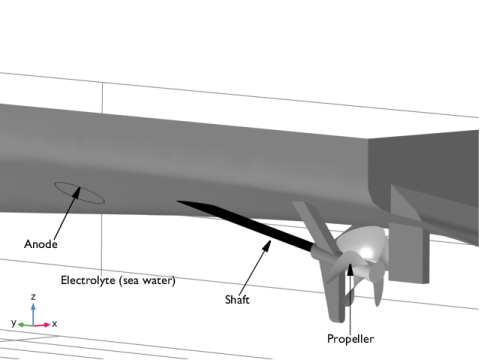
On the object fin, select Boundaries 8–11 and 14 only.
It might be easier to select the boundaries by using the Selection List window. To open this window, in the Home toolbar click Windows and choose Selection List. (If you are running the cross-platform desktop, you find Windows in the main menu.)
3
In the Geometry toolbar, click  Build All.
4
Click the  Transparency button in the Graphics toolbar.
5
Click the  Zoom Extents button in the Graphics toolbar.
The geometry should now look like Figure 1.
Select Zoom Box and a region closer to propeller. The zoomed in geometry should now look like Figure 2.
Global Definitions
Load the model parameters.
Parameters 1
1
In the Model Builder window, under Global Definitions click Parameters 1.
2
In the Settings window for Parameters, locate the Parameters section.
3
Click  Load from File.
4
Definitions
Create explicit selections for the propeller base, propeller blades, shaft, anode, reference electrode and hull surfaces. Then create a selection for the ship hull surface by using a union. The selections will be used later on when specifying the physics, setting up the mesh and when plotting and evaluating the results.
Propeller base
1
In the Definitions toolbar, click  Explicit.
2
In the Settings window for Explicit, locate the Input Entities section.
3
From the Geometric entity level list, choose Boundary.
4
Click  Paste Selection.
5
In the Paste Selection dialog box, type 20-22 in the Selection text field.
6
7
In the Settings window for Explicit, type Propeller base in the Label text field.
Propeller blades
1
In the Definitions toolbar, click  Explicit.
2
In the Settings window for Explicit, locate the Input Entities section.
3
From the Geometric entity level list, choose Boundary.
4
Click  Paste Selection.
5
In the Paste Selection dialog box, type 14,16,17,40,41 in the Selection text field.
6
7
In the Settings window for Explicit, type Propeller blades in the Label text field.
Shaft
1
In the Definitions toolbar, click  Explicit.
2
In the Settings window for Explicit, locate the Input Entities section.
3
From the Geometric entity level list, choose Boundary.
4
Click  Paste Selection.
5
In the Paste Selection dialog box, type 29,39 in the Selection text field.
6
7
In the Settings window for Explicit, type Shaft in the Label text field.
Anode
1
In the Definitions toolbar, click  Explicit.
2
In the Settings window for Explicit, locate the Input Entities section.
3
From the Geometric entity level list, choose Boundary.
4
Click  Paste Selection.
5
In the Paste Selection dialog box, type 19 in the Selection text field.
6
7
In the Settings window for Explicit, type Anode in the Label text field.
Reference electrode
1
In the Definitions toolbar, click  Explicit.
2
In the Settings window for Explicit, locate the Input Entities section.
3
From the Geometric entity level list, choose Boundary.
4
Click  Paste Selection.
5
In the Paste Selection dialog box, type 18 in the Selection text field.
6
7
In the Settings window for Explicit, type Reference electrode in the Label text field.
Hull surface
1
In the Definitions toolbar, click  Explicit.
2
In the Settings window for Explicit, locate the Input Entities section.
3
From the Geometric entity level list, choose Boundary.
4
Click  Paste Selection.
5
In the Paste Selection dialog box, type 6-13, 15, 20-28, 30-38, 42-47 in the Selection text field.
6
7
In the Settings window for Explicit, type Hull surface in the Label text field.
Ship surface
1
In the Definitions toolbar, click  Union.
2
In the Settings window for Union, locate the Geometric Entity Level section.
3
From the Level list, choose Boundary.
4
Locate the Input Entities section. Under Selections to add, click  Add.
5
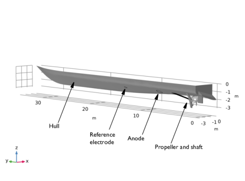
In the Add dialog box, in the Selections to add list, choose Propeller blades, Shaft, Anode, Reference electrode, and Hull surface.
6
7
In the Settings window for Union, type Ship surface in the Label text field.
Propeller and Shaft
1
In the Definitions toolbar, click  Union.
2
In the Settings window for Union, locate the Geometric Entity Level section.
3
From the Level list, choose Boundary.
4
Locate the Input Entities section. Under Selections to add, click  Add.
5
In the Add dialog box, in the Selections to add list, choose Propeller base, Propeller blades, and Shaft.
6
7
In the Settings window for Union, type Propeller and Shaft in the Label text field.
Propeller
1
In the Definitions toolbar, click  Union.
2
In the Settings window for Union, locate the Geometric Entity Level section.
3
From the Level list, choose Boundary.
4
Locate the Input Entities section. Under Selections to add, click  Add.
5
In the Add dialog box, in the Selections to add list, choose Propeller base and Propeller blades.
6
7
In the Settings window for Union, type Propeller in the Label text field.
Materials
Use the Corrosion Material Library to set up the material properties for the electrode kinetics at the shaft and propeller electrode surfaces.
Add Material
1
In the Home toolbar, click  Add Material to open the Add Material window.
2
Go to the Add Material window.
3
In the tree, select Corrosion>Nickel Alloys>Alloy 625 in seawater at 30 C.
4
Click Add to Component in the window toolbar.
Materials
Alloy 625 in seawater at 30 C (mat1)
1
In the Settings window for Material, locate the Geometric Entity Selection section.
2
From the Geometric entity level list, choose Boundary.
3
From the Selection list, choose Shaft.
4
In the Model Builder window, expand the Alloy 625 in seawater at 30 C (mat1) node.
Interpolation 1 (iloc_exp)
1
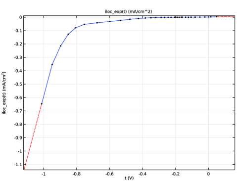
In the Model Builder window, expand the Component 1 (comp1)>Materials>Alloy 625 in seawater at 30 C (mat1)>Local current density (lcd) node, then click Interpolation 1 (iloc_exp).
2
In the Settings window for Interpolation, click  Plot.
The function plot should look like this:
Add Material
1
Go to the Add Material window.
2
In the tree, select Corrosion>Copper Alloys (Bronzes)>NAB in seawater at 30 C.
3
Click Add to Component in the window toolbar.
Materials
NAB in seawater at 30 C (mat2)
1
In the Settings window for Material, locate the Geometric Entity Selection section.
2
From the Geometric entity level list, choose Boundary.
3
From the Selection list, choose Propeller.
4
In the Model Builder window, expand the NAB in seawater at 30 C (mat2) node.
Interpolation 1 (iloc_exp)
1
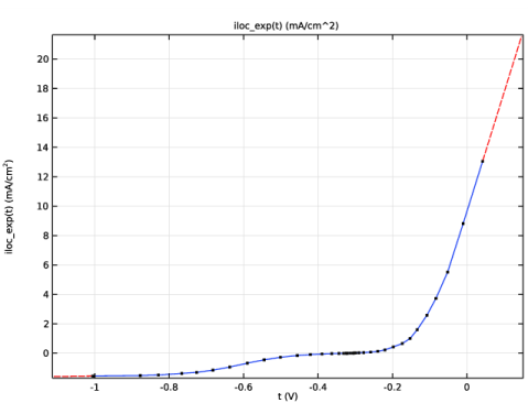
In the Model Builder window, expand the Component 1 (comp1)>Materials>NAB in seawater at 30 C (mat2)>Local current density (lcd) node, then click Interpolation 1 (iloc_exp).
2
In the Settings window for Interpolation, click  Plot.
The function plot should look like this:
3
In the Home toolbar, click  Add Material to close the Add Material window.
Cathodic Protection (cp)
Now, set up the Cathodic Protection interface for the case of a coated propeller.
Electrolyte 1
Set up the user defined electrolyte conductivity.
1
In the Settings window for Electrolyte, locate the Electrolyte section.
2
From the σl list, choose User defined. In the associated text field, type sigma.
Reference Electrode 1
The ICCP system will control the potential of the ship hull versus a reference electrode, located at midship. In this model we set all Equilibrium potential with reference to Ag/AgCl. The equilibrium potential of this reference is hence 0.
1
In the Model Builder window, right-click Cathodic Protection (cp) and choose Points>Reference Electrode.
2
Impressed Current Surface 1
In this model we will not explicitly define the anode reaction kinetics. Instead we will use a potential (primary) condition for the anode potential.
1
In the Physics toolbar, click  Boundaries and choose Impressed Current Surface.
2
In the Settings window for Impressed Current Surface, locate the Boundary Selection section.
3
From the Selection list, choose Anode.
4
Locate the Impressed Current Surface section. In the Eimpr text field, type E_control.
5
From the φs,ref list, choose Electric reference potential (cp/refel1).
Electrode Surface 1
Now specify the electrode potential and the kinetics for the shaft surface.
1
In the Physics toolbar, click  Boundaries and choose Electrode Surface.
2
In the Settings window for Electrode Surface, locate the Boundary Selection section.
3
From the Selection list, choose Shaft.
Electrode Reaction 1
1
In the Model Builder window, click Electrode Reaction 1.
2
In the Settings window for Electrode Reaction, locate the Electrode Kinetics section.
3
From the iloc,expr list, choose From material.
4
Select the Limiting current density check box.
5
In the ilim text field, type ilim.
Passive Metal Surface 1
Next set the insulation condition for the ship surface.
1
In the Physics toolbar, click  Boundaries and choose Passive Metal Surface.
2
In the Settings window for Passive Metal Surface, locate the Boundary Selection section.
3
From the Selection list, choose Hull surface.
Thin Passive Metal Surface 1
Next set the insulation condition for the propeller blade surface.
1
In the Physics toolbar, click  Boundaries and choose Thin Passive Metal Surface.
2
In the Settings window for Thin Passive Metal Surface, locate the Boundary Selection section.
3
From the Selection list, choose Propeller blades.
Add an Infinite Electrolyte to describe an infinite extension of the electrolyte. Use symmetry planes to describe the ocean surface and the midship symmetry planes.
Infinite Electrolyte 1
1
In the Physics toolbar, click  Boundaries and choose Infinite Electrolyte.
2
3
In the Settings window for Infinite Electrolyte, locate the Electrolyte section.
4
In the σl text field, type sigma.
5
Click to expand the Symmetry Planes section. Select the yz-plane check box.
6
Select the xy-plane check box.
No more boundary conditions are needed for study with the coated propeller since Insulation condition is applied by default, including the coated propeller surfaces.
Initial Values 1
Provide an initial value for the electrolyte potential to reduce the computational time.
1
In the Model Builder window, click Initial Values 1.
2
In the Settings window for Initial Values, locate the Initial Values section.
3
In the phil text field, type 0.5.
Mesh 1
Build a mesh with a finer resolution at the propeller, shaft and hull surface. Mesh the domain around the propeller first.
Free Tetrahedral 1
1
In the Mesh toolbar, click  Free Tetrahedral.
2
In the Settings window for Free Tetrahedral, locate the Domain Selection section.
3
From the Geometric entity level list, choose Domain.
4
Size 1
1
Right-click Free Tetrahedral 1 and choose Size.
2
In the Settings window for Size, locate the Element Size section.
3
From the Predefined list, choose Extra fine.
4
Click the Custom button.
5
Locate the Element Size Parameters section.
6
Select the Maximum element size check box. In the associated text field, type 1.5.
7
Select the Minimum element size check box. In the associated text field, type 0.01.
Size 2
1
In the Model Builder window, right-click Free Tetrahedral 1 and choose Size.
2
In the Settings window for Size, locate the Geometric Entity Selection section.
3
From the Geometric entity level list, choose Boundary.
4
From the Selection list, choose Propeller and Shaft.
5
Locate the Element Size section. From the Predefined list, choose Fine.
Size 3
1
Right-click Free Tetrahedral 1 and choose Size.
2
In the Settings window for Size, locate the Geometric Entity Selection section.
3
From the Geometric entity level list, choose Boundary.
4
From the Selection list, choose Propeller base.
5
Locate the Element Size section. From the Predefined list, choose Extra fine.
6
Click  Build Selected.
Free Tetrahedral 2
In the Mesh toolbar, click  Free Tetrahedral.
Size 1
Right-click Free Tetrahedral 2 and choose Size.
Free Tetrahedral 2
1
In the Model Builder window, right-click Free Tetrahedral 2 and choose Build Selected.
The mesh should look like Figure 3 (You may want to toggle the transparency button in order to see the mesh better).
Study : Coated Propeller
Now, solve the model for the coated propeller case.
1
In the Model Builder window, click Study 1.
2
In the Settings window for Study, type Study : Coated Propeller in the Label text field.
3
In the Home toolbar, click  Compute.
Results
Several plots are added by default. Now, add a surface plot for hull potential to the electrode potential versus adjacent reference plot.
Electrode Potential vs. Adjacent Reference (cp)
1
In the Model Builder window, under Results click Electrode Potential vs. Adjacent Reference (cp).
2
In the Settings window for 3D Plot Group, locate the Plot Settings section.
3
Clear the Plot dataset edges check box.
4
Locate the Color Legend section. From the Position list, choose Left.
5
In the Electrode Potential vs. Adjacent Reference (cp) toolbar, click  Plot.
The surface plot of the potential for the ship surface with the coated propeller should look like Figure 5.
Surface 1
In the Model Builder window, expand the Electrolyte Current Density (cp) node, then click Surface 1.
Selection 1
1
In the Electrolyte Current Density (cp) toolbar, click  Selection.
2
In the Settings window for Selection, locate the Selection section.
3
From the Selection list, choose Shaft.
4
In the Electrolyte Current Density (cp) toolbar, click  Plot.
Electrolyte Current Density (cp)
Select Zoom Box and a region closer to propeller. The surface plot of the total current density for the zoomed in region near the coated propeller should look like Figure 6.
Cathodic Protection (cp)
Now, set up the problem for an uncoated propeller case by describing the electrode kinetics at the propeller base surfaces using the Electrode Surface boundary feature and at the propeller blade surfaces using the Thin Electrode Surface boundary feature.
Electrode Surface 2
1
In the Physics toolbar, click  Boundaries and choose Electrode Surface.
2
In the Settings window for Electrode Surface, locate the Boundary Selection section.
3
From the Selection list, choose Propeller base.
Electrode Reaction 1
1
In the Model Builder window, click Electrode Reaction 1.
2
In the Settings window for Electrode Reaction, locate the Electrode Kinetics section.
3
From the iloc,expr list, choose From material.
4
Select the Limiting current density check box.
5
In the ilim text field, type ilim.
Thin Electrode Surface 1
1
In the Physics toolbar, click  Boundaries and choose Thin Electrode Surface.
2
In the Settings window for Thin Electrode Surface, locate the Boundary Selection section.
3
From the Selection list, choose Propeller blades.
Electrode Reaction 1
1
In the Model Builder window, click Electrode Reaction 1.
2
In the Settings window for Electrode Reaction, locate the Electrode Kinetics section.
3
From the iloc,expr list, choose From material.
4
Select the Limiting current density check box.
5
In the ilim text field, type ilim.
Study : Coated Propeller
Now, disable the Electrode Surface 2 and Thin Electrode Surface 1 boundary nodes in study for the coated propeller and add a new study to solve the model for the uncoated propeller case.
Step 1: Stationary
1
In the Model Builder window, under Study : Coated Propeller click Step 1: Stationary.
2
In the Settings window for Stationary, locate the Physics and Variables Selection section.
3
Select the Modify model configuration for study step check box.
4
In the tree, select Component 1 (comp1)>Cathodic Protection (cp)>Electrode Surface 2.
5
6
In the tree, select Component 1 (comp1)>Cathodic Protection (cp)>Thin Electrode Surface 1.
7
Add Study
1
In the Home toolbar, click  Add Study to open the Add Study window.
2
Go to the Add Study window.
3
Find the Studies subsection. In the Select Study tree, select General Studies>Stationary.
4
Click Add Study in the window toolbar.
5
In the Home toolbar, click  Add Study to close the Add Study window.
Click Add Study again to close the Add Study frame.
Study : Uncoated Propeller
1
In the Model Builder window, click Study 2.
2
In the Settings window for Study, type Study : Uncoated Propeller in the Label text field.
3
In the Home toolbar, click  Compute.
Results
Several plots are added by default for the uncoated propeller case. The surface plot of the total current density for the zoomed in region near the uncoated propeller should look like Figure 8. Now, add a surface plot for hull potential to the electrode potential versus adjacent reference plot.
Electrode Potential vs. Adjacent Reference (cp) 1
1
In the Model Builder window, under Results click Electrode Potential vs. Adjacent Reference (cp) 1.
2
In the Settings window for 3D Plot Group, locate the Plot Settings section.
3
Clear the Plot dataset edges check box.
4
Locate the Color Legend section. From the Position list, choose Left.
5
Click the  Zoom Extents button in the Graphics toolbar.
6
In the Electrode Potential vs. Adjacent Reference (cp) 1 toolbar, click  Plot.
The surface plot of the potential for the ship surface with the uncoated propeller should look like Figure 7.
Potential Along Keel
Now, create a Line Plot along the keel of the hull potential for both the coated and uncoated propeller cases.
1
In the Home toolbar, click  Add Plot Group and choose 1D Plot Group.
2
In the Settings window for 1D Plot Group, type Potential Along Keel in the Label text field.
3
Locate the Data section. From the Dataset list, choose None.
Line Graph 1
1
Right-click Potential Along Keel and choose Line Graph.
2
In the Settings window for Line Graph, locate the Data section.
3
From the Dataset list, choose Study : Coated Propeller/Solution 1 (sol1).
4
5
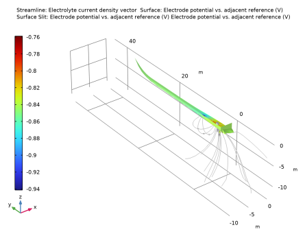
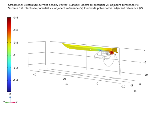
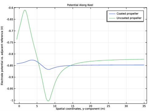
Click Replace Expression in the upper-right corner of the y-Axis Data section. From the menu, choose Component 1 (comp1)>Cathodic Protection>cp.Evsref - Electrode potential vs. adjacent reference - V.
6
Locate the x-Axis Data section. From the Parameter list, choose Expression.
7
In the Expression text field, type y.
8
Click to expand the Legends section. Select the Show legends check box.
9
From the Legends list, choose Manual.
10
Line Graph 2
1
Right-click Line Graph 1 and choose Duplicate.
2
In the Settings window for Line Graph, locate the Data section.
3
From the Dataset list, choose Study : Uncoated Propeller/Solution 2 (sol2).
4
Locate the Legends section. In the table, enter the following settings:
Potential Along Keel
1
In the Model Builder window, click Potential Along Keel.
2
In the Settings window for 1D Plot Group, click to expand the Title section.
3
From the Title type list, choose Label.
4
In the Potential Along Keel toolbar, click  Plot.
The potential comparison plot for the coated and uncoated propellers should look like Figure 9.
Global Evaluation 1
Finally, evaluate the magnitude of the current imposed by the ICCP anode.
1
In the Results toolbar, click  Global Evaluation.
2
In the Settings window for Global Evaluation, click Replace Expression in the upper-right corner of the Expressions section. From the menu, choose Component 1 (comp1)>Cathodic Protection>cp.Itot_imprcs1 - Total impressed current - A.
3
Click  Evaluate.
Global Evaluation 2
1
Right-click Global Evaluation 1 and choose Duplicate.
2
In the Settings window for Global Evaluation, locate the Data section.
3
From the Dataset list, choose Study : Uncoated Propeller/Solution 2 (sol2).
4
Click  Evaluate.