
|
|
|
|
•
|
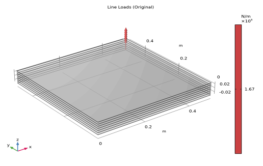
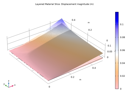
A total load of 1 kN is applied to one of the corners of the right end of the laminate in the form of a line load as shown in Figure 2.
|
|
•
|
|
•
|
|
1
|
|
2
|
|
3
|
Click Add.
|
|
4
|
Click
|
|
5
|
|
6
|
Click
|
|
1
|
|
2
|
|
3
|
|
4
|
Browse to the model’s Application Libraries folder and double-click the file stacking_sequence_optimization_parameters.txt.
|
|
1
|
In the Model Builder window, under Component 1 (comp1)>Layered Shell (lshell) click Linear Elastic Material 1.
|
|
2
|
|
3
|
|
1
|
In the Model Builder window, under Global Definitions right-click Materials and choose Blank Material.
|
|
2
|
|
1
|
|
2
|
|
4
|
Click
|
|
6
|
Click
|
|
8
|
|
1
|
|
2
|
|
3
|
|
4
|
|
5
|
|
6
|
|
1
|
In the Model Builder window, under Component 1 (comp1) right-click Materials and choose Layers>Layered Material Link.
|
|
2
|
|
3
|
|
4
|
Click to expand the Preview Plot Settings section. In the Thickness-to-width ratio text field, type 0.4.
|
|
5
|
Click Section_bar in the upper-right corner of the Layered Material Settings section. From the menu, choose Layer Cross-Section Preview.
|
|
6
|
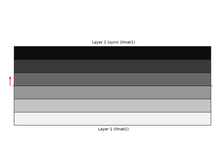
Click Section_bar in the upper-right corner of the Layered Material Settings section. From the menu, choose Layer Stack Preview.
|
|
1
|
In the Model Builder window, under Global Definitions>Materials click Material: Carbon-Epoxy (mat1).
|
|
2
|
|
1
|
|
1
|
|
3
|
|
4
|
|
5
|
|
1
|
|
2
|
|
3
|
|
1
|
|
2
|
|
1
|
|
2
|
|
3
|
|
1
|
|
2
|
|
4
|
Click
|
|
1
|
|
2
|
|
3
|
|
1
|
|
2
|
|
3
|
|
4
|
|
5
|
|
1
|
|
2
|
|
3
|
|
1
|
In the Model Builder window, expand the Stress, Slice (Original) node, then click Layered Material Slice 1.
|
|
2
|
|
3
|
|
4
|
|
5
|
|
6
|
|
7
|
|
8
|
|
9
|
|
10
|
|
1
|
|
2
|
|
3
|
|
4
|
|
5
|
|
1
|
|
2
|
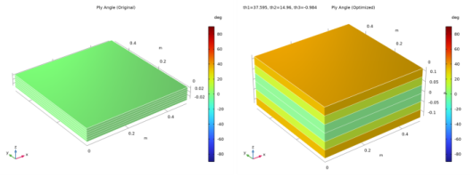
In the tree, select Study 1: Original Layup/Solution 1 (sol1)>Layered Shell>Geometry and Layup (lshell)>Ply Angle (lshell).
|
|
3
|
|
4
|
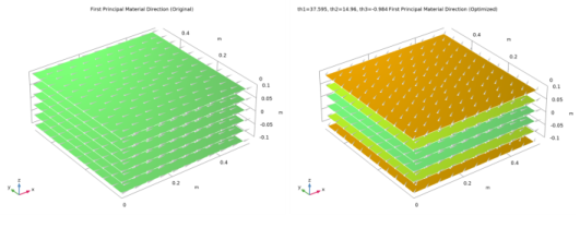
In the tree, select Study 1: Original Layup/Solution 1 (sol1)>Layered Shell>Geometry and Layup (lshell)>First Principal Material Direction (lshell).
|
|
5
|
|
1
|
|
2
|
|
3
|
|
1
|
|
2
|
|
3
|
|
1
|
|
2
|
|
3
|
|
4
|
|
1
|
|
2
|
|
3
|
|
1
|
|
2
|
|
3
|
|
1
|
|
2
|
In the Settings window for 3D Plot Group, type First Principal Material Direction (Original) in the Label text field.
|
|
3
|
|
1
|
|
2
|
In the tree, select Study 1: Original Layup/Solution 1 (sol1)>Layered Shell>Applied Loads (lshell)>Line Loads (lshell).
|
|
3
|
|
1
|
|
2
|
|
1
|
|
2
|
|
3
|
|
4
|
|
5
|
|
1
|
|
2
|
|
1
|
|
2
|
|
3
|
|
4
|
|
5
|
|
7
|
Click
|
|
9
|
Click
|
|
11
|
|
1
|
|
2
|
|
3
|
|
1
|
|
2
|
|
3
|
|
4
|
|
1
|
|
2
|
In the tree, select Study 2: Layup Optimization/Parametric Solutions 1 (sol3)>Layered Shell>Stress, Slice (lshell).
|
|
3
|
|
1
|
In the Model Builder window, expand the Stress, Slice (Optimized) node, then click Layered Material Slice 1.
|
|
2
|
|
3
|
|
4
|
|
5
|
|
6
|
|
7
|
|
8
|
|
1
|
|
2
|
|
3
|
|
4
|
|
1
|
|
2
|
In the tree, select Study 2: Layup Optimization/Parametric Solutions 1 (sol3)>Layered Shell>Geometry and Layup (lshell)>Ply Angle (lshell).
|
|
3
|
|
4
|
In the tree, select Study 2: Layup Optimization/Parametric Solutions 1 (sol3)>Layered Shell>Geometry and Layup (lshell)>First Principal Material Direction (lshell).
|
|
5
|
|
6
|
|
1
|
|
2
|
|
3
|
|
1
|
|
2
|
|
3
|
|
1
|
|
2
|
|
3
|
|
4
|
|
1
|
|
2
|
|
3
|
|
1
|
|
2
|
|
3
|
|
1
|
|
2
|
In the Settings window for 3D Plot Group, type First Principal Material Direction (Optimized) in the Label text field.
|
|
3
|
|
1
|
In the Model Builder window, expand the Stress, Slice (Original) 1 node, then click Layered Material Slice 1.
|
|
2
|
|
3
|
|
4
|
|
5
|
Locate the Through-Thickness Location section. From the Location definition list, choose Reference surface.
|
|
6
|
|
7
|
|
8
|
|
9
|
|
10
|
Click OK.
|
|
11
|
|
12
|
Select the Wireframe check box.
|
|
1
|
|
2
|
|
3
|
|
4
|
|
5
|
|
6
|
|
1
|
In the Model Builder window, expand the Results>Stress, Slice (Original) 1>Layered Material Slice 1 node, then click Deformation.
|
|
2
|
|
3
|
|
1
|
|
2
|
In the Settings window for 3D Plot Group, type Displacement: Original and Optimized in the Label text field.
|
|
3
|
|
4
|
|
5
|