PDF

Progressive Delamination in a Laminated Shell
Introduction
Interfacial failure or delamination in a composite material can be simulated with a cohesive zone model (CZM). A key ingredient of a cohesive zone model is a traction-separation law that describes the softening in the cohesive zone near the delamination tip. This example shows the implementation of a CZM with a bilinear traction-separation law in a laminated composites using the Layered Shell interface. The capabilities of the CZM to predict mixed-mode softening and delamination propagation are demonstrated in the model.
The example illustrates the delamination initiation and propagation in a composite plate having two layers with an initial delaminated region at the interface. A compressive load is gradually applied and removed in a parametric study in order to predict the total interfacial damage in one load cycle.
Model Definition
The geometry of a composite plate is shown in Figure 1. The composite plate consists of two layers where each layer has a thickness of 1.5 mm with [0/45] stacking sequence.
Figure 1: The geometry of a composite plate having two layers with an initial delaminated region at the interface.
The geometry consists of circular regions where the interface between the two layers is in delaminated or debonded state.
Material Properties
The material properties are those of AS4/PEEK unidirectional laminates. The orthotropic linear elastic properties assume that the longitudinal direction is aligned with the global X direction. The material properties of the laminate composite are listed in Table 1.
EX
EY=EZ
νYZ
νXY=νXZ
GYZ
GXY=GXZ
Cohesive Zone Model (CZM)
The CZM used in this example is defined using the displacement based damage model available in the Delamination node. The model is used to predict crack propagation at the interface of a laminated composite under different loading. The material properties needed for this constitutive model are summarized in Table 2.
σt
σs
pn
106 N/mm3
GIc
GIIc
η
The CZM is defined using a bilinear traction-separation law. Traction increases linearly with a stiffness pn until the opening crack reaches a damage initiation displacement u0. When the crack opens beyond u0, the material softens irreversibly and the stiffness decreases as a function of increasing damage d. The material fails once the stiffness has decreased to zero, that is, when d = 1. This happens at the ultimate displacement uf.
The values of u0 and uf depend on whether the separation displacement is normal (mode I) or tangential (mode II and III) to an interface. For the mixed mode, a combination is used. For the displacement based damage model, two different criteria are available to define this combination. Here the model by Benzeggagh and Kenane is used.
Boundary conditions
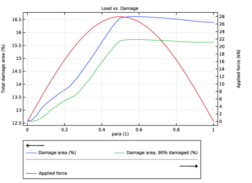
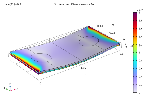
Face load with a total maximum value of 28 kN is applied at the top surface of the composite plate in negative z-direction. The load is parametrically increased and then decreased to zero using a sinusoidal function.
Finite element mesh
A rather fine mapped mesh is used in the geometry in order to accurately predict the initiation and propagation of delamination in the structure.
Figure 2: A mapped finite element mesh used to accurately model the delamination propagation in the composite plate.
In the thickness direction, each layer has only one mesh element in order to reduce the overall computation time.
Results and Discussion
The von Mises stress distribution in both layers of the composite plate when the applied load is having maximum value is shown in Figure 3. The corresponding von Mises stress distribution at the midplane of two layers is shown in Figure 4. In this figure, the bottom layer undergoes higher stresses than the top layer due to the bending effects and fiber orientation.
Figure 3: von Mises stress distribution in the composite plate for maximum applied force value.
The state of delaminated region when the applied load is having maximum value is shown in Figure 5, where debonded part is shown in red and bonded part is shown in green color. It can be seen the delamination starts near the comparatively weaker regions or high stress regions. The two such locations in the plate are the boundaries of initially delaminated region and the region near fixed edges.
The adhesive stress in the first tangent direction when the applied load is having maximum value is shown in Figure 6. Figure 7 illustrates the variation of applied load and total damage area as a function of parameter. It can be seen that the interfacial damage is irreversible and it stays permanently in the structure even if the load is removed. In the plot there are two damage area indices plotted; one is the overall damage area index and the other is the damage area index where the interface has broken by 90% or more.
Figure 4: von Mises stress distribution at layer midplanes for maximum applied force value.
Figure 5: Plot showing the health of the laminate interface for maximum applied force value. The debonded part is shown in red, the intact part in green.
Figure 6: Adhesive stress in first tangent direction for maximum applied force value.
Figure 7: Load vs. damage curve. The overall damage area as well as area where 90% or more damage has occurred are shown.
Notes About the COMSOL Implementation
To implement a cohesive zone model in Layered Shell interface, use the Delamination node which allows you to model adhesion, delamination and contact after delamination. There are two different ways to specify adhesive stiffness with default being taken from the interface material properties. Cohesive zone models are based on either displacement or energy in order to predict the interfacial separation. The contact after delamination is modeled by penalty contact method.
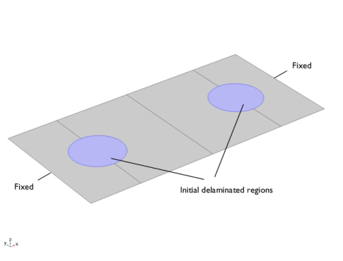
The Delamination node can be used to model already delaminated region by setting initial state to delaminated. To model the portion of interface which is not delaminated set the initial state to bonded.
The Delamination node is only applicable to the internal interfaces of composite laminates.
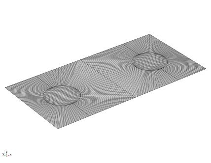
Modeling a composite laminated shell requires a surface geometry (2D), in general called a base surface, and a Layered Material node which adds an extra dimension (1D) to the base surface geometry in the surface normal direction. You can use the Layered Material functionality to model several layers stacked on top of each other having different thicknesses, material properties, and fiber orientations. You can also optionally specify the interface materials between the layers and control mesh elements in each layer.
Application Library path: Composite_Materials_Module/Delamination/progressive_delamination_in_a_laminated_shell
Modeling Instructions
From the File menu, choose New.
New
In the New window, click  Model Wizard.
Model Wizard
1
In the Model Wizard window, click  3D.
2
In the Select Physics tree, select Structural Mechanics>Layered Shell (lshell).
3
Click Add.
4
Click  Study.
5
In the Select Study tree, select General Studies>Stationary.
6
Global Definitions
Parameters 1
1
In the Model Builder window, under Global Definitions click Parameters 1.
2
In the Settings window for Parameters, locate the Parameters section.
3
Click  Load from File.
4
Browse to the model’s Application Libraries folder and double-click the file progressive_delamination_in_a_laminated_shell_parameters.txt.
AS4/PEEK
1
In the Model Builder window, under Global Definitions right-click Materials and choose Blank Material.
2
In the Settings window for Material, type AS4/PEEK in the Label text field.
Add a Layered Material node and assign appropriate thickness and rotation angles to each ply.
Layered Material: [0/45]
1
Right-click Materials and choose Layered Material.
2
In the Settings window for Layered Material, type Layered Material: [0/45] in the Label text field.
3
Locate the Layer Definition section. In the table, enter the following settings:
4
5
Definitions
Variables 1
1
In the Model Builder window, under Component 1 (comp1) right-click Definitions and choose Variables.
2
In the Settings window for Variables, locate the Variables section.
3
The geometry is in an XY-plane in which the fibers are oriented with respect to the X direction. Hence set the first axis of the laminate coordinate system in the X direction. Also set the frame of Boundary System to reference configuration.
Boundary System 1 (sys1)
1
In the Model Builder window, click Boundary System 1 (sys1).
2
In the Settings window for Boundary System, locate the Settings section.
3
From the Frame list, choose Reference configuration.
4
Find the Coordinate names subsection. From the Axis list, choose x.
Geometry 1
Work Plane 1 (wp1)
In the Geometry toolbar, click  Work Plane.
Work Plane 1 (wp1)>Plane Geometry
In the Model Builder window, click Plane Geometry.
Work Plane 1 (wp1)>Rectangle 1 (r1)
1
In the Work Plane toolbar, click  Rectangle.
2
In the Settings window for Rectangle, locate the Size and Shape section.
3
In the Width text field, type lb/2.
4
In the Height text field, type wb.
5
Click  Build Selected.
6
Click the  Zoom Extents button in the Graphics toolbar.
Work Plane 1 (wp1)>Circle 1 (c1)
1
In the Work Plane toolbar, click  Circle.
2
In the Settings window for Circle, locate the Size and Shape section.
3
In the Radius text field, type lb/10.
4
Locate the Position section. In the xw text field, type lb/5.
5
In the yw text field, type wb/2.
Work Plane 1 (wp1)>Rectangle 2 (r2)
1
In the Work Plane toolbar, click  Rectangle.
2
In the Settings window for Rectangle, locate the Size and Shape section.
3
In the Width text field, type lb/5.
4
In the Height text field, type wb.
5
Click  Build Selected.
Work Plane 1 (wp1)>Mirror 1 (mir1)
1
In the Work Plane toolbar, click  Transforms and choose Mirror.
2
Click in the Graphics window and then press Ctrl+A to select all objects.
3
In the Settings window for Mirror, locate the Input section.
4
Select the Keep input objects check box.
5
Locate the Point on Line of Reflection section. In the xw text field, type lb/2.
6
Click  Build Selected.
Form Union (fin)
In the Home toolbar, click  Build All.
Ignore Edges 1 (ige1)
1
In the Model Builder window, right-click Geometry 1 and choose Virtual Operations>Ignore Edges.
2
On the object fin, select Edges 8 and 20 only.
3
In the Geometry toolbar, click  Build All.
Materials
Layered Material Link 1 (llmat1)
In the Model Builder window, under Component 1 (comp1) right-click Materials and choose Layers>Layered Material Link.
Global Definitions
AS4/PEEK (mat1)
1
In the Settings window for Material, locate the Material Contents section.
2
Layered Shell (lshell)
For the portion of interface which is initially delaminated, the initial state in Delamination node can be set to Delaminated.
Delamination 1
1
In the Model Builder window, under Component 1 (comp1) right-click Layered Shell (lshell) and choose Material Models>Delamination.
2
3
In the Settings window for Delamination, locate the Initial State section.
4
5
Locate the Contact section. In the pn text field, type pn.
Delamination 2
For the portion of interface which is not yet delaminated, the initial state in Delamination node can be set to Bonded. To model contact between delaminated interfaces, the penalty factor is taken same as adhesive stiffness.
1
In the Physics toolbar, click  Boundaries and choose Delamination.
2
3
In the Settings window for Delamination, locate the Adhesion section.
4
From the Adhesive stiffness list, choose User defined.
5
Specify the kA vector as
6
Locate the Delamination section. In the σt text field, type N_strength.
7
In the σs text field, type S_strength.
8
In the Gct text field, type GIc.
9
In the Gcs text field, type GIIc.
10
From the Mixed mode criterion list, choose Benzeggagh-Kenane.
11
In the α text field, type eta.
12
Locate the Contact section. From the Penalty factor list, choose From adhesive stiffness.
Fixed Constraint 1
1
In the Physics toolbar, click  Edges and choose Fixed Constraint.
2
Face Load 1
1
In the Physics toolbar, click  Boundaries and choose Face Load.
2
In the Settings window for Face Load, locate the Boundary Selection section.
3
From the Selection list, choose All boundaries.
4
Locate the Interface Selection section. From the Apply to list, choose Top interface.
5
Locate the Force section. From the Load type list, choose Total force.
6
Specify the Ftot vector as
Mesh 1
Mapped 1
1
In the Mesh toolbar, click  Boundary and choose Mapped.
2
In the Settings window for Mapped, locate the Boundary Selection section.
3
From the Selection list, choose All boundaries.
Distribution 1
1
Right-click Mapped 1 and choose Distribution.
2
3
In the Settings window for Distribution, locate the Distribution section.
4
In the Number of elements text field, type 25.
5
In the Model Builder window, right-click Mesh 1 and choose Build All.
Study 1
Step 1: Stationary
1
In the Model Builder window, under Study 1 click Step 1: Stationary.
2
In the Settings window for Stationary, locate the Study Settings section.
3
Select the Include geometric nonlinearity check box.
4
Click to expand the Study Extensions section. Select the Auxiliary sweep check box.
5
6
Solution 1 (sol1)
1
In the Study toolbar, click  Show Default Solver.
2
In the Model Builder window, expand the Solution 1 (sol1) node.
Switch to an undamped Newton method.
3
In the Model Builder window, expand the Study 1>Solver Configurations>Solution 1 (sol1)>Stationary Solver 1 node, then click Fully Coupled 1.
4
In the Settings window for Fully Coupled, click to expand the Method and Termination section.
5
From the Nonlinear method list, choose Constant (Newton).
6
In the Study toolbar, click  Compute.
Results
Stress (lshell)
1
In the Settings window for 3D Plot Group, locate the Data section.
2
From the Parameter value (para) list, choose 0.5.
Surface 1
1
In the Model Builder window, expand the Stress (lshell) node, then click Surface 1.
2
In the Settings window for Surface, locate the Expression section.
3
From the Unit list, choose MPa.
4
Click to expand the Range section. Select the Manual color range check box.
5
In the Minimum text field, type 0.
6
In the Maximum text field, type 2e3.
Stress (lshell)
In the Model Builder window, collapse the Results>Stress (lshell) node.
Root
1
In the Model Builder window, right-click the root node and choose Plot.
2
In the Home toolbar, click  Add Predefined Plot.
Add Predefined Plot
1
Go to the Add Predefined Plot window.
2
In the tree, select Study 1/Solution 1 (sol1)>Layered Shell>Stress, Slice (lshell).
3
Click Add Plot in the window toolbar.
4
In the Home toolbar, click  Add Predefined Plot.
Results
Stress, Slice (lshell)
1
In the Model Builder window, under Results click Stress, Slice (lshell).
2
In the Settings window for 3D Plot Group, locate the Data section.
3
From the Parameter value (para) list, choose 0.5.
4
Locate the Plot Settings section. Clear the Plot dataset edges check box.
Layered Material Slice 1
1
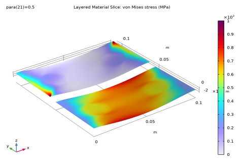
In the Model Builder window, expand the Stress, Slice (lshell) node, then click Layered Material Slice 1.
2
In the Settings window for Layered Material Slice, locate the Through-Thickness Location section.
3
From the Location definition list, choose Layer midplanes.
4
Locate the Layout section. From the Displacement list, choose Linear.
5
From the Orientation list, choose y.
6
Locate the Expression section. From the Unit list, choose MPa.
7
Click to expand the Range section. Select the Manual color range check box.
8
In the Minimum text field, type 0.
9
In the Maximum text field, type 1e3.
Interface Health, 100% Damaged
1
In the Home toolbar, click  Add Plot Group and choose 3D Plot Group.
2
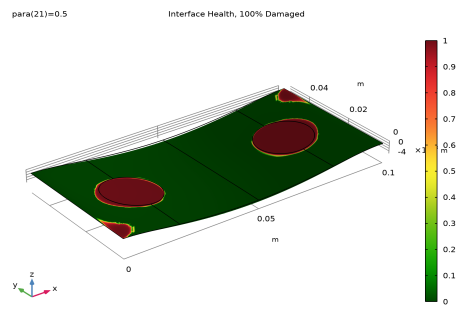
In the Settings window for 3D Plot Group, type Interface Health, 100% Damaged in the Label text field.
3
Locate the Data section. From the Parameter value (para) list, choose 0.5.
4
Locate the Plot Settings section. From the Frame list, choose Spatial  (x, y, z).
5
Click to expand the Title section. From the Title type list, choose Label.
Layered Material Slice 1
1
In the Interface Health, 100% Damaged toolbar, click  More Plots and choose Layered Material Slice.
2
In the Settings window for Layered Material Slice, locate the Expression section.
3
In the Expression text field, type lshell.idmg.
4
Locate the Through-Thickness Location section. From the Location definition list, choose Interfaces.
5
Locate the Coloring and Style section. Click  Change Color Table.
6
In the Color Table dialog box, select Traffic>Traffic in the tree.
7
Deformation 1
1
Right-click Layered Material Slice 1 and choose Deformation.
2
In the Settings window for Deformation, locate the Scale section.
3
Select the Scale factor check box. In the associated text field, type 1.
Interface Health, 100% Damaged
In the Model Builder window, collapse the Results>Interface Health, 100% Damaged node.
Root
1
In the Model Builder window, right-click the root node and choose Plot.
2
Click the  Zoom Extents button in the Graphics toolbar.
Results
Interface Health, 90% Damaged
1
In the Model Builder window, right-click Interface Health, 100% Damaged and choose Duplicate.
2
In the Settings window for 3D Plot Group, type Interface Health, 90% Damaged in the Label text field.
Layered Material Slice 1
1
In the Model Builder window, expand the Interface Health, 90% Damaged node, then click Layered Material Slice 1.
2
In the Settings window for Layered Material Slice, locate the Expression section.
3
In the Expression text field, type lshell.idmg>=0.9.
Interface Health, 90% Damaged
1
In the Model Builder window, collapse the Results>Interface Health, 90% Damaged node.
2
In the Model Builder window, click Interface Health, 90% Damaged.
3
In the Interface Health, 90% Damaged toolbar, click  Plot.
Adhesive Stress, t1 Direction
1
In the Home toolbar, click  Add Plot Group and choose 3D Plot Group.
2
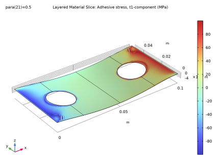
In the Settings window for 3D Plot Group, type Adhesive Stress, t1 Direction in the Label text field.
3
Locate the Data section. From the Parameter value (para) list, choose 0.5.
4
Locate the Plot Settings section. From the Frame list, choose Spatial  (x, y, z).
Layered Material Slice 1
1
In the Adhesive Stress, t1 Direction toolbar, click  More Plots and choose Layered Material Slice.
2
In the Settings window for Layered Material Slice, click Replace Expression in the upper-right corner of the Expression section. From the menu, choose Component 1 (comp1)>Layered Shell>Delamination>Adhesive stress (spatial frame) - N/m²>lshell.fst1 - Adhesive stress, t1-component.
3
Locate the Expression section. From the Unit list, choose MPa.
4
Locate the Through-Thickness Location section. From the Location definition list, choose Interfaces.
5
Locate the Coloring and Style section. Click  Change Color Table.
6
In the Color Table dialog box, select Rainbow>RainbowLight in the tree.
7
8
In the Settings window for Layered Material Slice, locate the Coloring and Style section.
9
From the Scale list, choose Linear symmetric.
Deformation 1
1
Right-click Layered Material Slice 1 and choose Deformation.
2
In the Settings window for Deformation, locate the Scale section.
3
Select the Scale factor check box. In the associated text field, type 1.
Adhesive Stress, t1 Direction
1
In the Model Builder window, collapse the Results>Adhesive Stress, t1 Direction node.
2
In the Model Builder window, click Adhesive Stress, t1 Direction.
3
In the Adhesive Stress, t1 Direction toolbar, click  Plot.
Layered Material (Interfaces)
1
In the Results toolbar, click  More Datasets and choose Layered Material.
2
In the Settings window for Layered Material, type Layered Material (Interfaces) in the Label text field.
3
Locate the Layers section. From the Evaluate in list, choose Interfaces.
4
In the Model Builder window, collapse the Results>Datasets node.
Surface Integration 1
1
In the Results toolbar, click  More Derived Values and choose Integration>Surface Integration.
2
In the Settings window for Surface Integration, locate the Data section.
3
From the Dataset list, choose Layered Material (Interfaces).
4
Locate the Selection section. From the Selection list, choose All boundaries.
5
Locate the Expressions section. In the table, enter the following settings:
6
Click  Evaluate.
Load vs. Damage
1
In the Results toolbar, click  1D Plot Group.
2
In the Settings window for 1D Plot Group, type Load vs. Damage in the Label text field.
3
Click to expand the Title section. From the Title type list, choose Label.
4
Locate the Plot Settings section.
5
Select the x-axis label check box. In the associated text field, type para (1).
6
Select the y-axis label check box. In the associated text field, type Total damage area (%).
7
Select the Two y-axes check box.
8
Click to collapse the Axis section. Locate the Legend section. From the Layout list, choose Outside graph axis area.
9
From the Position list, choose Bottom.
Table Graph 1
1
Right-click Load vs. Damage and choose Table Graph.
2
In the Settings window for Table Graph, click to expand the Legends section.
3
Select the Show legends check box.
Global 1
1
In the Model Builder window, right-click Load vs. Damage and choose Global.
2
In the Settings window for Global, locate the Data section.
3
From the Dataset list, choose Study 1/Solution 1 (sol1).
4
Locate the y-Axis section. Select the Plot on secondary y-axis check box.
5
Locate the y-Axis Data section. In the table, enter the following settings:
Load vs. Damage
1
In the Model Builder window, collapse the Results>Load vs. Damage node.
2
In the Model Builder window, click Load vs. Damage.
3
In the Load vs. Damage toolbar, click  Plot.
Animation: Stress
1
In the Results toolbar, click  Animation and choose Player.
2
In the Settings window for Animation, type Animation: Stress in the Label text field.
3
Locate the Frames section. From the Frame selection list, choose All.
4
Locate the Playing section. In the Display each frame for text field, type 0.3.
Animation: Interface Health
1
Right-click Animation: Stress and choose Duplicate.
2
In the Settings window for Animation, type Animation: Interface Health in the Label text field.
3
Locate the Scene section. From the Subject list, choose Interface Health, 100% Damaged.
Animation: Adhesive Stress
1
Right-click Animation: Interface Health and choose Duplicate.
2
In the Settings window for Animation, type Animation: Adhesive Stress in the Label text field.
3
Locate the Scene section. From the Subject list, choose Adhesive Stress, t1 Direction.