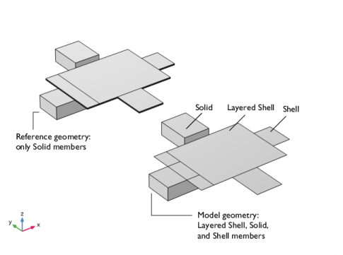
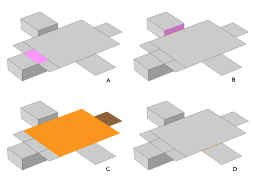
You are viewing the documentation for an older COMSOL version. The latest version is available here.
PDF

Connecting Layered Shells with Solids and Shells
Introduction
The Layered Shell interface is used to model thick to moderately thin composite laminates. These composite laminates are often connected with solid or sufficiently thin structures in different configurations to represent a realistic structure. These solid and thin structures are in general accurately and efficiently modeled using Solid Mechanics and Shell interfaces respectively.
This tutorial and verification model illustrates how to connect layered shell elements with solid and shell elements in cladding or side-by-side configuration using built-in coupling features. In this example, the results of the layered shell-solid-shell structure is compared with the reference model built using solid elements.
Model Definition
The model (Figure 1) consists of two set of geometries; model geometry and reference geometry. The model geometry consists of layered shell, solid, and shell members whereas the reference geometry is modeled with only solid members.
Figure 1: The model and reference geometry showing different structural members in different parts of the geometry.
layered Shell-Structure Couplings
The model geometry has three sections. The middle section is modeled as a layered shell member, while side supports are modeled using solid and shell members as shown in Figure 1. The model geometry is made up of solid blocks and surfaces whereas the reference geometry is made up of only solid blocks. The connection between the layered shell and other structural members are defined as below:
Figure 2: Different connections of layered shell with other structural members on different sides are as follows:(A) layered shell-solid cladding (B) layered shell-solid transition (C) layered shell-shell cladding (D) layered shell-shell transition.
Stacking Sequence
In the model geometry, layered shell and shell members consist of two layers where each layer (ply) has a thickness of 10 mm with [0/45] stacking sequence.
Note that in case of layered shell-solid transition coupling, only bottom layer of layered shell is connected to the solid whereas top layer is set to free. Similar connection is achieved in the reference model by slitting the degrees of freedom using Thin Elastic Layer node in the Solid Mechanics interface.
Material Properties
In the model geometry, layered shell and shell members are made up of carbon-epoxy composite material. The homogenized transversely isotropic material properties (Young’s modulus, shear modulus, and Poisson’s ratio) are given in Table 1 and density of the lamina is taken as 1700 kg/m3.
{E1,E2}
{G12}
{υ12,υ23}
The solid members in the model geometry are made up of structural steel. The stacking sequence and materials in the reference geometry are used as per the model geometry specifications.
Boundary conditions
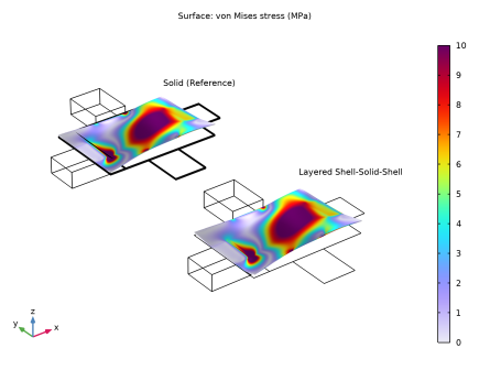
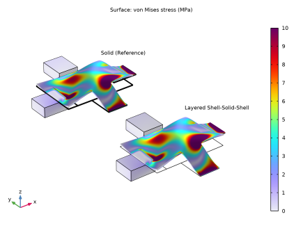
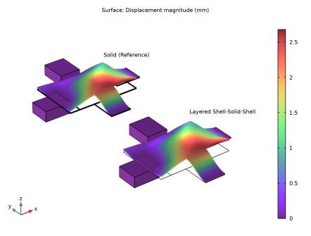
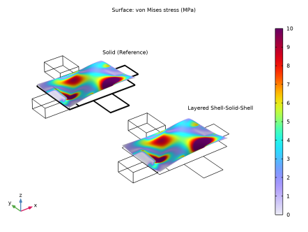
Boundary load of 10 kN is applied at the top surface of the middle plate modeled using layered shell.
Results and Discussion
von Mises stress distribution for the given applied load is shown in Figure 3. The stress distribution in the model geometry matches quite well with the same in the reference geometry. The total displacement in both setups are shown in Figure 4 which also matches quite closely with each other. This shows the accuracy of different types of elements and connections used in the model geometry.
Figure 3: The comparison of von Mises stress distribution in both structural models.
The distribution of von Mises stress in the bottom and top layer of composite laminate modeled using layered shell and solid elements are shown in Figure 5 and Figure 6, respectively.
The distribution of von Mises stress at the common edge between layered shell and different structural members is also compared with the reference model. Figure 7 through Figure 10 illustrate such a comparison with a good overall qualitative and quantitative match.
Figure 4: The comparison of total displacement distribution in both structural models.
Figure 5: The comparison of von Mises stress distribution in the bottom layer of both structural models.
Figure 6: The comparison of von Mises stress distribution in the top layer of both structural models.
Figure 7: von Mises stress along the common edge for layered shell-solid cladding coupling.
Figure 8: von Mises stress along the common edge for layered shell-shell cladding coupling.
Figure 9: von Mises stress along the common edge for layered shell-shell transition coupling.
Figure 10: von Mises stress along the common edge for layered shell-solid transition coupling.
Notes About the COMSOL Implementation
Modeling a composite laminate requires a surface geometry (2D), in general called a base surface, and a Layered Material node, which adds an extra dimension (1D) to the base surface geometry in the surface normal direction. You can use the Layered Material functionality to model several layers stacked on top of each other having different thicknesses, material properties, and fiber orientations. Optionally, you can also specify the interface materials between the layers and control mesh elements in each layer.
From a constitutive model point of view, you can either use the Layerwise (LW) theory based Layered Shell interface or the Equivalent Single Layer (ESL) theory based Layered Linear Elastic Material node in the Shell interface.
The Layered Shell - Structure Cladding multiphysics coupling is used to model cladding between a Layered Shell interface and a Solid Mechanics, Shell or Membrane interface. In the Connection Settings section, shared and parallel boundaries options are provided to connect boundaries of different structural physics interfaces.
The Layered Shell - Structure Transition multiphysics coupling is used to couple side-by-side structural connection between a Layered Shell interface and a Solid Mechanics or Shell interface. This is a layered multiphysics coupling and in the Shell Properties section, it is possible to select only few layers for the connection.
Application Library path: Composite_Materials_Module/Tutorials/layered_shell_structure_connection
Modeling Instructions
From the File menu, choose New.
New
In the New window, click  Model Wizard.
Model Wizard
1
In the Model Wizard window, click  3D.
2
In the Select Physics tree, select Structural Mechanics>Solid Mechanics (solid), Structural Mechanics>Shell (shell), and Structural Mechanics>Layered Shell (lshell).
3
4
Click  Study.
5
In the Select Study tree, select General Studies>Stationary.
6
Layered Shell (lshell)
In the Model Builder window, under Component 1 (comp1) right-click Layered Shell (lshell) and choose Move Up.
Global Definitions
Parameters 1
1
In the Model Builder window, under Global Definitions click Parameters 1.
2
In the Settings window for Parameters, locate the Parameters section.
3
If you do not want to build all the geometry, you can load the geometry sequence from the stored model. In the Model Builder window, under Component 1 (comp1) right-click Geometry 1 and choose Insert Sequence. Browse to the model’s Application Libraries folder and double-click the file layered_shell_structure_connection.mph. You can then continue to the Definitions section below.
To build the geometry from scratch, continue here.
Geometry 1
Work Plane 1 (wp1)
In the Geometry toolbar, click  Work Plane.
Work Plane 1 (wp1)>Plane Geometry
In the Model Builder window, click Plane Geometry.
Work Plane 1 (wp1)>Rectangle 1 (r1)
1
In the Work Plane toolbar, click  Rectangle.
2
In the Settings window for Rectangle, locate the Size and Shape section.
3
In the Width text field, type 0.4*a.
4
In the Height text field, type 0.5*a.
5
Locate the Position section. In the xw text field, type 0.3*a.
6
In the yw text field, type -0.5*a.
Work Plane 1 (wp1)>Rotate 1 (rot1)
1
In the Work Plane toolbar, click  Transforms and choose Rotate.
2
3
In the Settings window for Rotate, locate the Input section.
4
Select the Keep input objects check box.
5
Locate the Rotation section. In the Angle text field, type 90 180 270.
6
Locate the Center of Rotation section. In the xw text field, type 0.5*a.
7
In the yw text field, type 0.5*a.
8
In the Work Plane toolbar, click  Build All.
Split 1 (spl1)
1
In the Model Builder window, right-click Geometry 1 and choose Conversions>Split.
2
In the Settings window for Split, locate the Input section.
3
Click  Paste Selection.
4
In the Paste Selection dialog box, type wp1 in the Selection text field.
5
6
In the Settings window for Split, click  Build Selected.
Extrude 1 (ext1)
1
In the Geometry toolbar, click  Extrude.
2
In the Settings window for Extrude, locate the General section.
3
From the Extrude from list, choose Faces.
4
On the object spl1(1), select Boundary 1 only.
5
On the object spl1(3), select Boundary 1 only.
6
Locate the Distances section. In the table, enter the following settings:
7
Select the Reverse direction check box.
8
Click  Build Selected.
Move 1 (mov1)
1
In the Geometry toolbar, click  Transforms and choose Move.
2
Select the object ext1(2) only.
3
In the Settings window for Move, locate the Displacement section.
4
In the z text field, type 10*th.
5
Click  Build Selected.
Move 2 (mov2)
1
In the Geometry toolbar, click  Transforms and choose Move.
2
Select the object spl1(4) only.
3
In the Settings window for Move, locate the Displacement section.
4
In the z text field, type -2*th.
5
Click  Build Selected.
Work Plane 2 (wp2)
In the Geometry toolbar, click  Work Plane.
Work Plane 2 (wp2)>Plane Geometry
In the Model Builder window, click Plane Geometry.
Work Plane 2 (wp2)>Rectangle 1 (r1)
1
In the Work Plane toolbar, click  Rectangle.
2
In the Settings window for Rectangle, locate the Size and Shape section.
3
In the Width text field, type 1.4*a.
4
In the Height text field, type a.
5
Locate the Position section. In the xw text field, type -0.2*a.
Work Plane 2 (wp2)>Rectangle 2 (r2)
1
In the Work Plane toolbar, click  Rectangle.
2
In the Settings window for Rectangle, locate the Size and Shape section.
3
In the Width text field, type 0.2*a.
4
In the Height text field, type a.
5
Locate the Position section. In the xw text field, type -0.2*a.
Move 3 (mov3)
1
In the Model Builder window, right-click Geometry 1 and choose Transforms>Move.
2
Click in the Graphics window and then press Ctrl+A to select all objects.
3
In the Settings window for Move, locate the Input section.
4
Select the Keep input objects check box.
5
Locate the Displacement section. In the y text field, type 2.5*a.
6
Click  Build Selected.
Extrude 2 (ext2)
1
In the Geometry toolbar, click  Extrude.
2
Click the  Zoom Extents button in the Graphics toolbar.
3
4
In the Settings window for Extrude, locate the General section.
5
From the Extrude from list, choose Faces.
6
On the object mov3(4), select Boundary 1 only.
7
On the object mov3(5), select Boundaries 1 and 2 only.
8
Locate the Distances section. In the table, enter the following settings:
9
Click  Build Selected.
Extrude 3 (ext3)
1
In the Geometry toolbar, click  Extrude.
2
In the Settings window for Extrude, locate the General section.
3
From the Extrude from list, choose Faces.
4
On the object mov3(3), select Boundary 1 only.
5
Locate the Distances section. In the table, enter the following settings:
6
Click  Build Selected.
Form Union (fin)
1
In the Geometry toolbar, click  Build All.
2
Click the  Show Grid button in the Graphics toolbar.
3
Click the  Go to Default View button in the Graphics toolbar.
Definitions
Variables 1
1
In the Model Builder window, under Component 1 (comp1) right-click Definitions and choose Variables.
2
In the Settings window for Variables, locate the Geometric Entity Selection section.
3
From the Geometric entity level list, choose Domain.
4
Click  Paste Selection.
5
In the Paste Selection dialog box, type 4,6 in the Selection text field.
6
7
In the Settings window for Variables, locate the Variables section.
8
Variables 2
1
In the Model Builder window, right-click Definitions and choose Variables.
2
In the Settings window for Variables, locate the Geometric Entity Selection section.
3
From the Geometric entity level list, choose Domain.
4
Click  Paste Selection.
5
In the Paste Selection dialog box, type 3,5 in the Selection text field.
6
7
In the Settings window for Variables, locate the Variables section.
8
Variables 3
1
Right-click Definitions and choose Variables.
2
In the Settings window for Variables, locate the Variables section.
3
Add required materials and layered material first.
Add Material
1
In the Home toolbar, click  Add Material to open the Add Material window.
2
Go to the Add Material window.
3
In the tree, select Built-in>Structural steel.
4
Right-click and choose Add to Global Materials.
5
In the Home toolbar, click  Add Material to close the Add Material window.
Global Definitions
Carbon-Epoxy
1
In the Model Builder window, under Global Definitions right-click Materials and choose Blank Material.
2
In the Settings window for Material, type Carbon-Epoxy in the Label text field.
Layered Material 1 (lmat1)
1
Right-click Materials and choose Layered Material.
2
In the Settings window for Layered Material, locate the Layer Definition section.
3
4
5
Materials
Layered Material Link 1 (llmat1)
1
In the Model Builder window, under Component 1 (comp1) right-click Materials and choose Layers>Layered Material Link.
2
In the Settings window for Layered Material Link, locate the Boundary Selection section.
3
Click  Clear Selection.
4
Click  Paste Selection.
5
In the Paste Selection dialog box, type 11-13, 25, 37, 69 in the Selection text field.
6
7
In the Settings window for Layered Material Link, locate the Orientation and Position section.
8
From the Position list, choose Bottom side on boundary.
Material Link 1 (matlnk1)
1
Right-click Materials and choose More Materials>Material Link.
2
In the Settings window for Material Link, locate the Geometric Entity Selection section.
3
Click  Paste Selection.
4
In the Paste Selection dialog box, type 3-6, 8, 9, 11, 12 in the Selection text field.
5
6
In the Settings window for Material Link, locate the Link Settings section.
7
From the Material list, choose Carbon-Epoxy (mat2).
Material Link 2 (matlnk2)
1
Right-click Materials and choose More Materials>Material Link.
2
In the Settings window for Material Link, locate the Geometric Entity Selection section.
3
Click  Paste Selection.
4
In the Paste Selection dialog box, type 1, 2, 7, 10 in the Selection text field.
5
Set linear elastic material in all physics interfaces to orthotropic. The isotropic properties of Structural Steel is automatically converted to orthotropic properties.
Set the discretization of Solid Mechanics interface to quadratic Lagrange in order to have a proper structural connection with other interfaces having quadratic Lagrange discretization.
Solid Mechanics (solid)
1
In the Model Builder window, under Component 1 (comp1) click Solid Mechanics (solid).
2
In the Settings window for Solid Mechanics, click to expand the Discretization section.
3
From the Displacement field list, choose Quadratic Lagrange.
Linear Elastic Material 1
1
In the Model Builder window, under Component 1 (comp1)>Solid Mechanics (solid) click Linear Elastic Material 1.
2
In the Settings window for Linear Elastic Material, locate the Linear Elastic Material section.
3
From the Material symmetry list, choose Orthotropic.
4
Select the Transversely isotropic check box.
Linear Elastic Material 2
1
In the Physics toolbar, click  Domains and choose Linear Elastic Material.
2
In the Settings window for Linear Elastic Material, locate the Linear Elastic Material section.
3
From the Material symmetry list, choose Orthotropic.
4
Select the Transversely isotropic check box.
5
Locate the Domain Selection section. Click  Paste Selection.
6
In the Paste Selection dialog box, type 4, 6, 9, 12 in the Selection text field.
7
Definitions (comp1)
Rotated System 2 (sys2)
1
In the Definitions toolbar, click  Coordinate Systems and choose Rotated System.
2
In the Settings window for Rotated System, locate the Rotation section.
3
Find the Euler angles (Z-X-Z) subsection. In the α text field, type pi/4.
Solid Mechanics (solid)
Linear Elastic Material 2
1
In the Model Builder window, under Component 1 (comp1)>Solid Mechanics (solid) click Linear Elastic Material 2.
2
In the Settings window for Linear Elastic Material, locate the Coordinate System Selection section.
3
From the Coordinate system list, choose Rotated System 2 (sys2).
To model the solid domains as disconnected, which are geometrically in union state, add Thin Elastic Layer node with zero stiffness.
Thin Elastic Layer 1
1
In the Physics toolbar, click  Boundaries and choose Thin Elastic Layer.
2
In the Settings window for Thin Elastic Layer, locate the Boundary Selection section.
3
Click  Paste Selection.
4
In the Paste Selection dialog box, type 57 in the Selection text field.
5
Boundary Load 1
1
In the Physics toolbar, click  Boundaries and choose Boundary Load.
2
3
In the Settings window for Boundary Load, locate the Force section.
4
From the Load type list, choose Total force.
5
Specify the Ftot vector as
Fixed Constraint 1
1
In the Physics toolbar, click  Boundaries and choose Fixed Constraint.
2
In the Settings window for Fixed Constraint, locate the Boundary Selection section.
3
Click  Paste Selection.
4
In the Paste Selection dialog box, type 1, 6, 43, 45, 48, 60, 82, 83 in the Selection text field.
5
Layered Shell (lshell)
1
In the Model Builder window, under Component 1 (comp1) click Layered Shell (lshell).
2
In the Settings window for Layered Shell, locate the Boundary Selection section.
3
Click  Clear Selection.
4
Click  Paste Selection.
5
In the Paste Selection dialog box, type 11-13, 25 in the Selection text field.
6
Face Load 1
In the Physics toolbar, click  Boundaries and choose Face Load.
Linear Elastic Material 1
1
In the Model Builder window, click Linear Elastic Material 1.
2
In the Settings window for Linear Elastic Material, locate the Linear Elastic Material section.
3
Select the Transversely isotropic check box.
Face Load 1
1
In the Model Builder window, click Face Load 1.
2
In the Settings window for Face Load, locate the Boundary Selection section.
3
From the Selection list, choose All boundaries.
4
Locate the Interface Selection section. From the Apply to list, choose Top interface.
5
Locate the Force section. From the Load type list, choose Total force.
6
Specify the Ftot vector as
Shell (shell)
1
In the Model Builder window, under Component 1 (comp1) click Shell (shell).
2
In the Settings window for Shell, locate the Boundary Selection section.
3
Click  Clear Selection.
4
Click  Paste Selection.
5
In the Paste Selection dialog box, type 37, 69 in the Selection text field.
6
Add Layered Linear Elastic Material to shell interface and set it to orthotropic.
Layered Linear Elastic Material 1
1
In the Physics toolbar, click  Boundaries and choose Layered Linear Elastic Material.
2
In the Settings window for Layered Linear Elastic Material, locate the Linear Elastic Material section.
3
From the Material symmetry list, choose Orthotropic.
4
Select the Transversely isotropic check box.
5
Locate the Boundary Selection section. Click  Paste Selection.
6
In the Paste Selection dialog box, type 37, 69 in the Selection text field.
7
Fixed Constraint 1
1
In the Physics toolbar, click  Edges and choose Fixed Constraint.
2
Multiphysics
Add different layered shell-structure multiphysics couplings for appropriate selections.
Layered Shell-Structure Cladding 1 (lssc1)
1
In the Physics toolbar, click  Multiphysics Couplings and choose Global>Layered Shell-Structure Cladding.
2
In the Settings window for Layered Shell-Structure Cladding, locate the Connection Settings section.
3
From the Layered shell boundary list, choose Bottom.
Layered Shell-Structure Transition 1 (lsst1)
1
In the Physics toolbar, click  Multiphysics Couplings and choose Edge>Layered Shell-Structure Transition.
2
3
In the Settings window for Layered Shell-Structure Transition, locate the Shell Properties section.
4
Clear the Use all layers check box.
5
In the Selection table, clear the check box for Layer 2.
6
Locate the Edge Selection section. Click  Clear Selection.
7
Click  Paste Selection.
8
In the Paste Selection dialog box, type 74 in the Selection text field.
9
10
In the Settings window for Layered Shell-Structure Transition, locate the Connection Settings section.
11
Select the Manual control of selections check box.
12
Locate the Boundary Selection, Solid section. Click  Clear Selection.
13
Click  Paste Selection.
14
In the Paste Selection dialog box, type 39, 41 in the Selection text field.
15
Layered Shell-Structure Cladding 2 (lssc2)
1
In the Physics toolbar, click  Multiphysics Couplings and choose Global>Layered Shell-Structure Cladding.
2
In the Settings window for Layered Shell-Structure Cladding, locate the Coupled Interfaces section.
3
From the Structure list, choose Shell (shell).
4
Locate the Connection Settings section. From the Connection type list, choose Parallel boundaries.
5
Locate the Boundary Selection, Layered Shell section. Click to select the  Activate Selection toggle button.
6
7
Locate the Boundary Selection, Structure section. Click to select the  Activate Selection toggle button.
8
9
Locate the Connection Settings section. From the Layered shell boundary list, choose Bottom.
10
From the Shell boundary list, choose Top.
Layered Shell-Structure Transition 2 (lsst2)
1
In the Physics toolbar, click  Multiphysics Couplings and choose Edge>Layered Shell-Structure Transition.
2
In the Settings window for Layered Shell-Structure Transition, locate the Coupled Interfaces section.
3
From the Structure list, choose Shell (shell).
4
Locate the Edge Selection section. Click  Clear Selection.
5
Now enter the orthotropic material properties of Carbon-Epoxy material.
Global Definitions
Carbon-Epoxy (mat2)
1
In the Model Builder window, under Global Definitions>Materials click Carbon-Epoxy (mat2).
2
In the Settings window for Material, locate the Material Contents section.
3
Mesh 1
Swept 1
In the Mesh toolbar, click  Swept.
Size
1
In the Model Builder window, click Size.
2
In the Settings window for Size, locate the Element Size section.
3
Click the Custom button.
4
Locate the Element Size Parameters section. In the Maximum element size text field, type 0.03.
5
In the Minimum element size text field, type 9.0E-4.
6
In the Maximum element growth rate text field, type 1.3.
7
In the Curvature factor text field, type 0.2.
8
In the Resolution of narrow regions text field, type 1.
Mapped 1
1
In the Mesh toolbar, click  Boundary and choose Mapped.
2
In the Settings window for Mapped, locate the Boundary Selection section.
3
Click  Paste Selection.
4
In the Paste Selection dialog box, type 11, 13, 25, 37, 69 in the Selection text field.
5
6
In the Settings window for Mapped, click  Build All.
Study 1
Switch off the generation of default plots, since for this study new custom plots are needed.
1
In the Model Builder window, click Study 1.
2
In the Settings window for Study, locate the Study Settings section.
3
Clear the Generate default plots check box.
4
In the Home toolbar, click  Compute.
As generation of default plots are switched off, create custom Layered Material datasets and plots.
Results
Layered Material 1
1
In the Model Builder window, expand the Results node.
2
Right-click Results>Datasets and choose More Datasets>Layered Material.
Layered Material: Bottom Layer
1
In the Results toolbar, click  More Datasets and choose Layered Material.
2
In the Settings window for Layered Material, locate the Layers section.
3
Find the Layer selection subsection. Clear the Use all layers check box.
4
5
In the Label text field, type Layered Material: Bottom Layer.
Layered Material: Top Layer
1
In the Results toolbar, click  More Datasets and choose Layered Material.
2
In the Settings window for Layered Material, type Layered Material: Top Layer in the Label text field.
3
Locate the Layers section. Find the Layer selection subsection. Clear the Use all layers check box.
4
5
In the Model Builder window, collapse the Results>Datasets node.
Stress
1
In the Results toolbar, click  3D Plot Group.
2
In the Settings window for 3D Plot Group, type Stress in the Label text field.
Surface 1
1
Right-click Stress and choose Surface.
2
In the Settings window for Surface, locate the Expression section.
3
In the Expression text field, type solid.mises.
4
From the Unit list, choose MPa.
5
Locate the Coloring and Style section. Click  Change Color Table.
6
In the Color Table dialog box, select Rainbow>Prism in the tree.
7
8
In the Settings window for Surface, click to expand the Range section.
9
Select the Manual color range check box.
10
In the Maximum text field, type 10.
Deformation 1
Right-click Surface 1 and choose Deformation.
Surface 2
1
In the Model Builder window, right-click Stress and choose Surface.
2
In the Settings window for Surface, locate the Data section.
3
From the Dataset list, choose Layered Material 1.
4
Locate the Expression section. In the Expression text field, type lshell.mises.
5
From the Unit list, choose MPa.
6
Click to expand the Title section. From the Title type list, choose None.
7
Click to expand the Inherit Style section. From the Plot list, choose Surface 1.
Deformation 1
1
Right-click Surface 2 and choose Deformation.
2
In the Settings window for Deformation, locate the Expression section.
3
In the x-component text field, type u3.
4
In the y-component text field, type v3.
5
In the z-component text field, type w3.
Surface 3
1
In the Model Builder window, right-click Stress and choose Surface.
2
In the Settings window for Surface, locate the Data section.
3
From the Dataset list, choose Layered Material 1.
4
Locate the Expression section. In the Expression text field, type shell.mises.
5
From the Unit list, choose MPa.
6
Locate the Title section. From the Title type list, choose None.
7
Locate the Inherit Style section. From the Plot list, choose Surface 1.
Deformation 1
1
Right-click Surface 3 and choose Deformation.
2
In the Settings window for Deformation, locate the Expression section.
3
In the x-component text field, type u2.
4
In the y-component text field, type v2.
5
In the z-component text field, type w2.
Stress
In the Model Builder window, under Results click Stress.
Table Annotation 1
1
In the Stress toolbar, click  More Plots and choose Table Annotation.
2
In the Settings window for Table Annotation, locate the Data section.
3
From the Source list, choose Local table.
4
5
Locate the Coloring and Style section. Clear the Show point check box.
Stress
1
In the Model Builder window, collapse the Results>Stress node.
2
In the Model Builder window, click Stress.
3
In the Stress toolbar, click  Plot.
4
Click the  Go to Default View button in the Graphics toolbar.
Displacement
1
Right-click Stress and choose Duplicate.
2
In the Settings window for 3D Plot Group, type Displacement in the Label text field.
Surface 1
1
In the Model Builder window, expand the Displacement node, then click Surface 1.
2
In the Settings window for Surface, locate the Expression section.
3
In the Expression text field, type solid.disp.
4
From the Unit list, choose mm.
5
Locate the Range section. Clear the Manual color range check box.
6
Locate the Coloring and Style section. Click  Change Color Table.
7
In the Color Table dialog box, select Rainbow>SpectrumLight in the tree.
8
Surface 2
1
In the Model Builder window, click Surface 2.
2
In the Settings window for Surface, locate the Expression section.
3
In the Expression text field, type lshell.disp.
4
From the Unit list, choose mm.
Surface 3
1
In the Model Builder window, click Surface 3.
2
In the Settings window for Surface, locate the Expression section.
3
In the Expression text field, type shell.disp.
4
From the Unit list, choose mm.
Displacement
1
In the Model Builder window, collapse the Results>Displacement node.
2
In the Model Builder window, click Displacement.
3
In the Displacement toolbar, click  Plot.
Stress: Layered Shell, Bottom Layer
1
In the Model Builder window, right-click Stress and choose Duplicate.
2
In the Settings window for 3D Plot Group, type Stress: Layered Shell, Bottom Layer in the Label text field.
Surface 3
1
In the Model Builder window, expand the Stress: Layered Shell, Bottom Layer node.
2
Right-click Results>Stress: Layered Shell, Bottom Layer>Surface 3 and choose Delete.
Surface 1
1
In the Model Builder window, under Results>Stress: Layered Shell, Bottom Layer click Surface 1.
2
In the Settings window for Surface, locate the Expression section.
3
In the Expression text field, type misesBot_solid.
Surface 2
1
In the Model Builder window, click Surface 2.
2
In the Settings window for Surface, locate the Data section.
3
From the Dataset list, choose Layered Material: Bottom Layer.
Stress: Layered Shell, Bottom Layer
1
In the Model Builder window, collapse the Results>Stress: Layered Shell, Bottom Layer node.
2
In the Model Builder window, click Stress: Layered Shell, Bottom Layer.
3
In the Stress: Layered Shell, Bottom Layer toolbar, click  Plot.
Stress: Layered Shell, Top Layer
1
Right-click Stress: Layered Shell, Bottom Layer and choose Duplicate.
2
In the Settings window for 3D Plot Group, type Stress: Layered Shell, Top Layer in the Label text field.
Surface 1
1
In the Model Builder window, expand the Stress: Layered Shell, Top Layer node, then click Surface 1.
2
In the Settings window for Surface, locate the Expression section.
3
In the Expression text field, type misesTop_solid.
Surface 2
1
In the Model Builder window, click Surface 2.
2
In the Settings window for Surface, locate the Data section.
3
From the Dataset list, choose Layered Material: Top Layer.
Stress: Layered Shell, Top Layer
1
In the Model Builder window, collapse the Results>Stress: Layered Shell, Top Layer node.
2
In the Model Builder window, click Stress: Layered Shell, Top Layer.
3
In the Stress: Layered Shell, Top Layer toolbar, click  Plot.
Stress, Layered Shell-Solid Cladding
1
In the Home toolbar, click  Add Plot Group and choose 1D Plot Group.
2
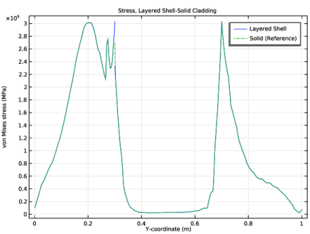
In the Settings window for 1D Plot Group, type Stress, Layered Shell-Solid Cladding in the Label text field.
3
Click to expand the Title section. From the Title type list, choose Label.
4
Locate the Plot Settings section.
5
Select the x-axis label check box. In the associated text field, type Y-coordinate (m).
6
Select the y-axis label check box. In the associated text field, type von Mises stress (MPa).
Line Graph 1
1
Right-click Stress, Layered Shell-Solid Cladding and choose Line Graph.
2
In the Settings window for Line Graph, locate the Selection section.
3
Click  Paste Selection.
4
In the Paste Selection dialog box, type 17, 19, 21 in the Selection text field.
5
6
In the Settings window for Line Graph, locate the y-Axis Data section.
7
In the Expression text field, type misesTop_lshell.
8
From the Unit list, choose MPa.
9
Click to expand the Legends section. Select the Show legends check box.
10
From the Legends list, choose Manual.
11
Line Graph 2
1
Right-click Line Graph 1 and choose Duplicate.
2
In the Settings window for Line Graph, locate the Selection section.
3
Click  Clear Selection.
4
Click  Paste Selection.
5
In the Paste Selection dialog box, type 30 in the Selection text field.
6
7
In the Settings window for Line Graph, locate the y-Axis Data section.
8
In the Expression text field, type solid.mises.
9
Click to expand the Coloring and Style section. Find the Line style subsection. From the Line list, choose Dashed.
10
Locate the Legends section. In the table, enter the following settings:
Stress, Layered Shell-Solid Cladding
1
In the Model Builder window, collapse the Results>Stress, Layered Shell-Solid Cladding node.
2
In the Model Builder window, click Stress, Layered Shell-Solid Cladding.
3
In the Stress, Layered Shell-Solid Cladding toolbar, click  Plot.
Stress, Layered Shell-Shell Cladding
1
Right-click Stress, Layered Shell-Solid Cladding and choose Duplicate.
2
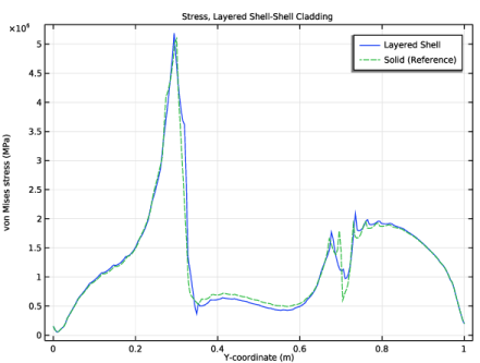
In the Settings window for 1D Plot Group, type Stress, Layered Shell-Shell Cladding in the Label text field.
Line Graph 1
1
In the Model Builder window, expand the Stress, Layered Shell-Shell Cladding node, then click Line Graph 1.
2
In the Settings window for Line Graph, locate the Selection section.
3
Click  Clear Selection.
4
Line Graph 2
1
In the Model Builder window, click Line Graph 2.
2
In the Settings window for Line Graph, locate the Selection section.
3
Click  Clear Selection.
4
5
Locate the x-Axis Data section. From the Parameter list, choose Reversed arc length.
Stress, Layered Shell-Shell Cladding
1
In the Model Builder window, collapse the Results>Stress, Layered Shell-Shell Cladding node.
2
In the Model Builder window, click Stress, Layered Shell-Shell Cladding.
3
In the Stress, Layered Shell-Shell Cladding toolbar, click  Plot.
Stress, Layered Shell-Shell Transition
1
Right-click Stress, Layered Shell-Shell Cladding and choose Duplicate.
2
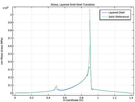
In the Settings window for 1D Plot Group, type Stress, Layered Shell-Shell Transition in the Label text field.
3
Locate the Plot Settings section.
4
Select the x-axis label check box. In the associated text field, type X-coordinate (m).
Line Graph 1
1
In the Model Builder window, expand the Stress, Layered Shell-Shell Transition node, then click Line Graph 1.
2
In the Settings window for Line Graph, locate the Selection section.
3
Click  Clear Selection.
4
Line Graph 2
1
In the Model Builder window, click Line Graph 2.
2
In the Settings window for Line Graph, locate the Selection section.
3
Click  Clear Selection.
4
Click  Paste Selection.
5
In the Paste Selection dialog box, type 31, 56, 92, 124 in the Selection text field.
6
7
In the Settings window for Line Graph, locate the x-Axis Data section.
8
From the Parameter list, choose Arc length.
Stress, Layered Shell-Shell Transition
1
In the Model Builder window, collapse the Results>Stress, Layered Shell-Shell Transition node.
2
In the Model Builder window, click Stress, Layered Shell-Shell Transition.
3
In the Stress, Layered Shell-Shell Transition toolbar, click  Plot.
Stress, Layered Shell-Solid Transition
1
Right-click Stress, Layered Shell-Shell Transition and choose Duplicate.
2
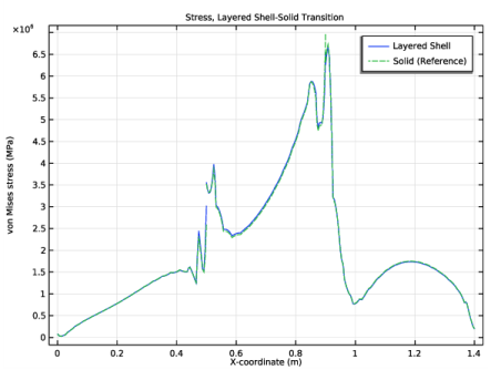
In the Settings window for 1D Plot Group, type Stress, Layered Shell-Solid Transition in the Label text field.
Line Graph 1
1
In the Model Builder window, expand the Stress, Layered Shell-Solid Transition node, then click Line Graph 1.
2
In the Settings window for Line Graph, locate the Selection section.
3
Click  Clear Selection.
4
Line Graph 2
1
In the Model Builder window, click Line Graph 2.
2
In the Settings window for Line Graph, locate the y-Axis Data section.
3
In the Expression text field, type misesTop_solid.
4
Locate the Selection section. Click  Clear Selection.
5
Click  Paste Selection.
6
In the Paste Selection dialog box, type 40, 66, 101, 132 in the Selection text field.
7
Stress, Layered Shell-Solid Transition
1
In the Model Builder window, collapse the Results>Stress, Layered Shell-Solid Transition node.
2
In the Model Builder window, click Stress, Layered Shell-Solid Transition.
3
In the Stress, Layered Shell-Solid Transition toolbar, click  Plot.