|
|
|


|
1
|
|
2
|
In the Select Physics tree, select Chemical Species Transport>Reacting Flow>Turbulent Flow>Turbulent Flow, k-ε.
|
|
3
|
Click Add.
|
|
4
|
|
5
|
|
6
|
In the Mass fractions table, enter the following settings:
|
|
7
|
|
8
|
Click Add.
|
|
9
|
Click
|
|
10
|
|
11
|
Click
|
|
1
|
|
2
|
|
3
|
|
4
|
Browse to the model’s Application Libraries folder and double-click the file polymerization_multijet_parameters.txt.
|
|
1
|
|
2
|
Browse to the model’s Application Libraries folder and double-click the file polymerization_multijet_geom_sequence.mph.
|
|
3
|
|
1
|
|
2
|
On the object fin, select Domain 4 only.
|
|
1
|
|
2
|
On the object mcd1, select Boundary 11 only.
|
|
1
|
|
2
|
|
3
|
|
4
|
|
1
|
In the Model Builder window, under Component 1 (comp1)>Turbulent Flow, k-ε (spf) click Fluid Properties 1.
|
|
2
|
|
3
|
From the μ list, choose User defined. In the associated text field, type 0.001*(1.17817558982837+(-298[K]+T)/223[K])^(-3.758)[Pa*s].
|
|
1
|
|
2
|
|
3
|
|
4
|
|
1
|
|
1
|
|
3
|
|
4
|
|
5
|
|
1
|
|
1
|
In the Model Builder window, under Component 1 (comp1) click Transport of Concentrated Species (tcs).
|
|
2
|
In the Settings window for Transport of Concentrated Species, locate the Transport Mechanisms section.
|
|
3
|
|
4
|
|
1
|
In the Model Builder window, under Component 1 (comp1)>Transport of Concentrated Species (tcs) click Species Molar Masses 1.
|
|
2
|
|
3
|
|
4
|
|
5
|
|
6
|
|
7
|
|
8
|
|
1
|
|
2
|
|
3
|
|
4
|
|
5
|
|
6
|
|
7
|
|
8
|
|
9
|
|
1
|
|
2
|
|
3
|
|
4
|
|
5
|
|
6
|
|
7
|
|
1
|
|
3
|
|
4
|
|
5
|
|
6
|
|
7
|
|
8
|
|
9
|
|
1
|
|
3
|
|
4
|
|
5
|
|
6
|
|
7
|
|
8
|
|
9
|
|
1
|
|
1
|
|
1
|
|
3
|
|
4
|
|
5
|
|
6
|
|
7
|
|
8
|
|
9
|
|
10
|
|
11
|
|
12
|
|
13
|
|
1
|
|
3
|
|
4
|
|
5
|
|
6
|
|
7
|
|
8
|
|
9
|
|
10
|
|
11
|
|
12
|
|
13
|
|
1
|
|
2
|
|
3
|
|
4
|
Locate the Heat Conduction, Fluid section. From the k list, choose User defined. In the associated text field, type 0.21+Cp_S*spf.muT/0.72.
|
|
5
|
|
6
|
|
7
|
|
8
|
|
1
|
|
2
|
|
3
|
|
1
|
|
3
|
|
4
|
|
1
|
|
1
|
|
1
|
|
3
|
|
4
|
|
1
|
|
2
|
|
3
|
|
1
|
|
2
|
|
3
|
|
1
|
|
2
|
|
3
|
|
5
|
|
6
|
|
1
|
|
2
|
|
3
|
|
1
|
|
2
|
|
3
|
|
4
|
|
5
|
|
1
|
|
2
|
|
3
|
|
1
|
|
3
|
|
4
|
|
5
|
|
6
|
|
1
|
|
2
|
|
3
|
In the table, clear the Solve for check boxes for Transport of Concentrated Species (tcs) and Heat Transfer in Fluids (ht).
|
|
4
|
|
1
|
|
2
|
|
3
|
In the table, clear the Solve for check boxes for Turbulent Flow, k-ε (spf) and Heat Transfer in Fluids (ht).
|
|
1
|
|
2
|
|
3
|
In the table, clear the Solve for check boxes for Turbulent Flow, k-ε (spf) and Transport of Concentrated Species (tcs).
|
|
4
|
|
1
|
|
2
|
|
3
|
|
4
|
|
5
|
|
1
|
|
2
|
|
3
|
|
4
|
|
5
|
|
6
|
|
7
|
|
8
|
|
9
|
|
10
|
Click
|
|
11
|
|
1
|
|
2
|
|
3
|
|
4
|
|
5
|
Click
|
|
1
|
|
2
|
|
3
|
|
4
|
|
5
|
Click
|
|
6
|
|
1
|
|
2
|
|
3
|
|
1
|
|
2
|
|
3
|
|
4
|
|
5
|
|
6
|
|
1
|
|
2
|
|
1
|
|
2
|
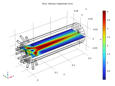
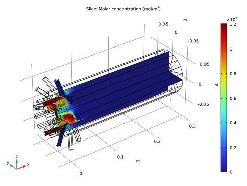
In the Settings window for Slice, click Replace Expression in the upper-right corner of the Expression section. From the menu, choose Component 1 (comp1)>Transport of Concentrated Species>Species wA>tcs.c_wA - Molar concentration - mol/m³.
|
|
3
|
|
1
|
|
2
|
|
3
|
|
4
|
|
5
|
|
6
|
|
7
|
|
8
|
|
1
|
|
2
|
|
1
|
|
2
|
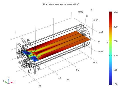
In the Settings window for Slice, click Replace Expression in the upper-right corner of the Expression section. From the menu, choose Component 1 (comp1)>Transport of Concentrated Species>Species wL>tcs.c_wL - Molar concentration - mol/m³.
|
|
3
|
|
1
|
|
2
|
|
3
|
|
1
|
|
2
|
|
1
|
|
2
|
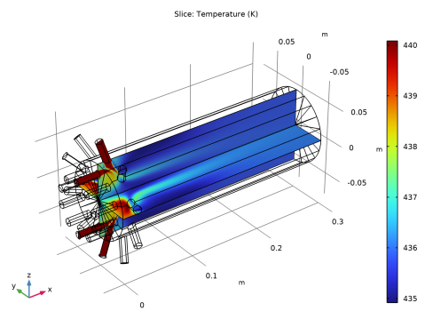
In the Settings window for Slice, click Replace Expression in the upper-right corner of the Expression section. From the menu, choose Component 1 (comp1)>Heat Transfer in Fluids>Temperature>T - Temperature - K.
|
|
1
|
|
2
|
In the Settings window for Slice, click Replace Expression in the upper-right corner of the Expression section. From the menu, choose Component 1 (comp1)>Heat Transfer in Fluids>Temperature>T - Temperature - K.
|
|
3
|
|
4
|
|
1
|
|
2
|
|
3
|
|
1
|
|
2
|
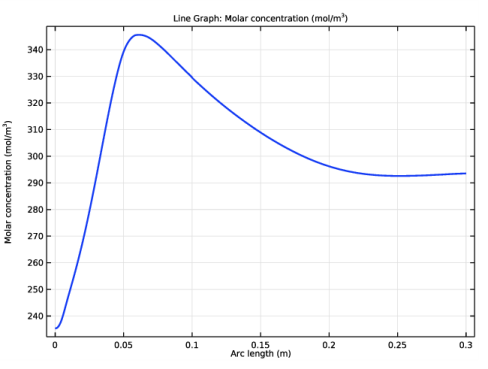
In the Settings window for Line Graph, click Replace Expression in the upper-right corner of the y-Axis Data section. From the menu, choose Component 1 (comp1)>Transport of Concentrated Species>Species wL>tcs.c_wL - Molar concentration - mol/m³.
|
|
3
|
|
4
|
|
5
|
|
1
|
|
2
|
|
3
|
|
1
|
|
2
|
|
3
|
|
4
|
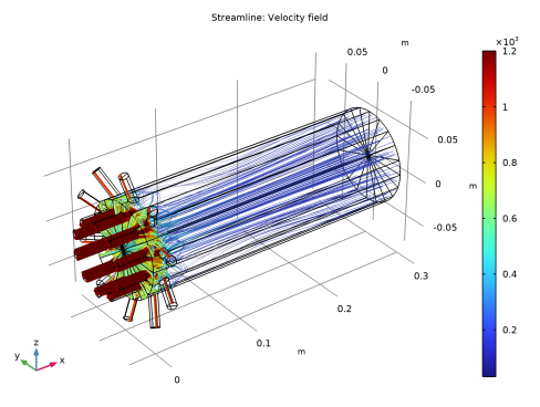
Locate the Coloring and Style section. Find the Line style subsection. From the Type list, choose Tube.
|
|
5
|
|
1
|
|
2
|
|
3
|
|
4
|
|
5
|
|
1
|
|
2
|
|
1
|
|
2
|
In the Settings window for 3D Plot Group, type Concentration, L (Isosurface) in the Label text field.
|
|
3
|
|
1
|
|
2
|
In the Settings window for Isosurface, click Replace Expression in the upper-right corner of the Expression section. From the menu, choose Component 1 (comp1)>Transport of Concentrated Species>Species wL>tcs.c_wL - Molar concentration - mol/m³.
|
|
3
|
|
4
|
|
5
|
|
1
|
|
2
|
|
3
|
|
4
|
|
5
|
|
6
|
|
7
|
|
8
|
From the gizmo context menu, select Align to y-Axis.
|
|
9
|
From the gizmo context menu, select Invert Clipping.
|
|
10
|
|
1
|
|
2
|
|
3
|
|
1
|
|
2
|
|
3
|
|
4
|
|
5
|
|
1
|
|
2
|
|
3
|
|
1
|
|
2
|
|
3
|
|
4
|
|
5
|
|
1
|
|
2
|
|
3
|
|
4
|
|
1
|
|
2
|
Click
|
|
1
|
|
2
|
|
3
|
|
4
|
|
5
|
|
6
|
|
7
|
|
1
|
|
3
|
Select the object cyl1 only.
|
|
4
|
|
5
|
|
6
|
|
7
|
|
8
|
|
9
|
|
1
|
|
2
|
|
3
|
|
4
|
|
5
|
|
6
|
|
7
|
|
8
|
|
1
|
|
2
|
On the object cyl2, select Boundary 4 only.
|
|
3
|
|
4
|
|
6
|
Click to expand the Scales section. In the table, enter the following settings:
|
|
7
|
|
1
|
|
2
|
Click in the Graphics window and then press Ctrl+A to select both objects.
|
|
3
|
|
4
|
|
5
|
|
1
|
|
2
|
|
3
|
|
1
|
|
2
|
Select the object uni1 only.
|
|
3
|
|
4
|
|
5
|
|
6
|
|
7
|
On the object par1, select Domain 2 only.
|
|
8
|
|
1
|
|
2
|
|
3
|
|
4
|
|
1
|
|
2
|
|
3
|
|
4
|
|
5
|
|
6
|
|
1
|
In the Model Builder window, under Component 1 (comp1)>Geometry 1 right-click Work Plane 2 (wp2) and choose Extrude.
|
|
2
|
|
4
|
|
1
|
|
2
|