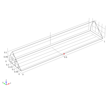
PDF

A Multiscale 3D Packed Bed Reactor
Introduction
The packed bed reactor is used in heterogeneous catalytic processes and is one of the most common reactors in the chemical industry. Its basic design is a column filled with porous catalyst particles, and in some cases the reactor also has a specially designed bottom plate through which the reaction mixture enters. The catalyst particles can be contained within a supporting structure, such as tubes or channels, or they can be packed in one single compartment in the reactor.
Figure 1: An example of the macroscale (bed volume with entry holes) and the microscale (pellet) of a packed bed reactor.
The bed with the packed catalyst particles makes the modeling of mass transport and reactions in the reactor a challenge. The challenge is that species transport and reaction occur in dimensions of different orders of magnitude:
As such, the problem is regarded as a multiscale problem. The Reactive Pellet Bed feature, available with the Transport of Diluted Species interface, is dedicated to these multiscale problems.
The structure between particles in the bed is described as a macroporous material of meter dimensions. The particle radii are often in the order of mm. The pores inside the catalyst particles form the microscale structure of the bed. The pore radii in the particles are often between 1 and 10 microns. There are two porosities that are important: bed porosity (macroscale) and pellet porosity (microscale). Sometimes such models are called double-porosity models.
When a pressure drop is applied across the bed, flow and convection of the fluid is initiated in the bed. The transport of chemicals inside the pellets are dominated by diffusion.
This model is an extension to the 1D example, Packed Bed Reactor, which contains more complex reactions.
Model Definition
A model geometry made up of one eighth of the reactor in Figure 1 can be used due to symmetry. The geometry is shown in Figure 2.
Figure 2: The packed bed reactor simulation geometry. Due to symmetry an 1/8 of the true geometry is modeled. The results will be expanded to the true geometry with aid of a sector data set.
The pressure drop in the reactor is modeled using the Darcy’s Law interface.
A reversible catalytic chemical reaction occurs inside the pellets. The reactant species A and B forms a product C:
A + B 2C
The reaction kinetics are assumed to be equimolecular and are set up with the Chemistry interface. The automatic reaction rate can thus be used and has the following form:
where k is the rate factor (SI unit: m3/(mol·s)) with the superscripts f and r denoting the forward and reverse reaction, respectively. ci is the concentration (SI unit: mol/m3) of species i. The forward reaction constant is defined with the inbuilt Arrhenius expression and the reverse is computed with the equilibrium constant of the reaction.
The mass transport of the reacting species in the reactor is modeled with the Transport of Diluted Species interface, which accounts for diffusion, convection, and reaction in diluted solutions. The species are assumed to be diluted in water.
The reaction inside the pellets is added to the mass balances in the Transport of Diluted Species interface with the Reactive Pellet Bed feature. This feature has a predefined extra dimension (1D) on the normalized radius (r = rdim/rpe) of the pellet particle. The mesh on the extra dimension has a default of 10 elements with a cubic root sequence distribution. If spherical pellets are selected, the following spherical diffusion/reaction equation is set up and solved along the pellet radius for each species i:
(1)
Here, r is a dimensionless radial coordinate that goes from 0 (center) to 1 (pellet surface), rpe is the pellet radius, and N the number of pellets per unit volume of bed. The advantage of formulating Equation 1 on a dimensionless 1D geometry is that the pellet radius can be changed without changing the geometry limits.
Dpe is an effective diffusion coefficient (SI unit: m2/s) and Rpe, i is the reaction source term (SI unit: mol/(m3·s)). Note that the latter term is taken per unit volume of porous pellet material.
At the pellet-fluid interface, a film condition assumption is made. The flux of mass across the pellet-fluid interface into the pellet is possibly rate determined by the resistance to mass transfer on the bulk fluid side. The resistance is expressed in terms of a film mass transfer coefficient, hDi, such that:
(2),
where Ni, inward is the molar flux from the free fluid into a pellet and has the SI unit moles/(m2·s). The mass transfer coefficient is defined in terms of the Sherwood number
(3)
In this model the Frössling correlation is used
(4)
It is applicable for mass transfer from spherical particles and relates the Sherwood number to the pellet Reynolds number and the Schmidt number
(5), ,
Here U is fluid velocity in the bed and ν is the kinematic viscosity of the fluid.
In Table 1 the model parameters are tabulated.
Hr
1 [m]
Rr
ρb
ρpe
εb
1-ρb/ρpe
εpe
rpe
Dpe,A
Dpe,B
2e-9 [m2/s]
Dpe,C
2e12 [m3/(mol s)]
Keq0
CA,in
CB,in
CC,in
DA
1e-8 [m2/s]
DB
1.5e-8 [m2/s]
DC
0.5e-8 [m2/s]
pDarcy
Results and Discussion
The following figures display the results at 180 s. Figure 3 shows the velocity distribution in the fluid between the pellets.
Figure 3: Velocity distribution on the macroscale.
Figure 4 shows the macroscale concentration of the reactant A in the bed column fluid. The species is consumed due to the catalytic chemical reaction in the pellets.
Figure 4: Concentration of reactant A.
Streamline plots can be useful to get an understanding of the flow pattern. It can be seen from Figure 5 that no recirculation occurs downstream from the entry holes. The fluid is evenly spread out in the bed chamber shortly after entering from through the bottom plate.
Figure 5: The streamlines show how the fluid enters the holes and then spread out in the bed volume as it. The colors of the lines represent the reactant concentration in moles/m3.
A line plot of the concentration inside a pellet at a certain position in the bed is useful in order to understand the kinetics at that point. Here a sampling point on the symmetry axis half way through the reactor (at x = 0.5, z = 0, y = 0) is used. The point is shown in Figure 6. and. In Figure 7 line plots of the reactants and the product inside a pellet at the sampling point is shown. Species A and B originates in bed pores and diffuses into the porous pellet, while at the same time forming species C. The diffusion coefficient of B is higher than that of A, leading to a higher concentration of B in the pellet center.
Figure 6: The position where the pellet plot is evaluated: Centerline of reactor at a height of 0.5 m.
Figure 7: Species concentration within the pellet, in the at the end of the simulation (t = 180 s).
It is also valuable to simultaneously compare the development in the micro scale and the macro scale. This is done in Figure 8 where the pellet concentration of species A is visualized using on spherical pellets in a regular grid pattern. For comparison, the bed concentration of the same species is also plotted on a cut plane through the reactor.
Figure 8: Concentration of species A in the reactor. The spheres show the pellet concentration in the corresponding positions. The development in the pellets can be compared to the bed concentration plotted on a cut plane.
In Figure 9 a line plot is used to evaluate the development in the reactor. Here the bed concentrations and the average pellet concentrations are plotted against the reactor height. It can be noted that species A and B exhibit a very similar development though the reactor. The inlet concentration of species C is zero, but inside the pellets significant levels of C is produced already at the inlet.
Figure 9: Species concentrations in the reactor bed as well as averaged pellet concentrations, plotted along the reactor height.
Application Library path: Chemical_Reaction_Engineering_Module/Reactors_with_Porous_Catalysts/packed_bed_reactor_3d
Modeling Instructions
Start by adding the necessary physics interfaces for a 3D model.
From the File menu, choose New.
New
In the New window, click  Model Wizard.
Model Wizard
1
In the Model Wizard window, click  3D.
2
In the Select Physics tree, select Chemical Species Transport>Chemistry (chem).
3
Click Add.
4
In the Select Physics tree, select Chemical Species Transport>Transport of Diluted Species in Porous Media (tds).
5
Click Add.
6
In the Number of species text field, type 3.
7
In the Concentrations table, enter the following settings:
8
In the Select Physics tree, select Fluid Flow>Porous Media and Subsurface Flow>Darcy’s Law (dl).
9
Click Add.
10
Click  Study.
11
In the Select Study tree, select General Studies>Time Dependent.
12
Global Definitions
Parameters 1
Add the model parameters from a text file.
1
In the Model Builder window, under Global Definitions click Parameters 1.
2
In the Settings window for Parameters, locate the Parameters section.
3
Click  Load from File.
4
Geometry 1
Now create the geometry. You can simplify this by inserting a prepared geometry sequence from a file with prepared geometry selections.
1
In the Model Builder window, expand the Component 1 (comp1)>Definitions node.
2
Right-click Component 1 (comp1)>Geometry 1 and choose Insert Sequence.
3
4
In the Geometry toolbar, click  Build All.
Create a global material. Some properties can be found in the COMSOL built-in materials, other are manually entered.
Assume the reaction mixture has mainly aqueous properties.
Add Material
1
In the Home toolbar, click  Add Material to open the Add Material window.
2
Go to the Add Material window.
3
In the tree, select Built-in>Water, liquid.
4
Click Add to Global Materials in the window toolbar.
5
In the Home toolbar, click  Add Material to close the Add Material window.
Define a porous material for the Reactive Pellet Bed feature.
Materials
Porous Material 1 (pmat1)
In the Model Builder window, under Component 1 (comp1) right-click Materials and choose More Materials>Porous Material.
Pellet 1 (pmat1.pellet1)
1
In the Model Builder window, right-click Porous Material 1 (pmat1) and choose Pellet.
Enter the properties of the reactive pellet bed.
2
In the Settings window for Pellet, locate the Pellet Properties section.
3
From the Material list, choose Locally defined.
4
In the dpe text field, type r_pe*2.
5
In the εpe text field, type epsilon_pe.
6
Locate the Pellet Bed Properties section. In the εp text field, type epsilon_b.
7
Click to expand the Mesh section. From the Distribution list, choose Linear.
8
In the Number of elements text field, type 12.
Fluid 1 (pmat1.fluid1)
In the Model Builder window, right-click Porous Material 1 (pmat1) and choose Fluid.
Transport of Diluted Species in Porous Media (tds)
Packed Bed 1
Add the Packed Bed feature. A extra dimension from porous material is attached to this feature. The extra dimension is 1D on the radial coordinate of the pellet particle of which the radius is normalized to 1. The mesh for the extra dimension has a default of 6 elements with a cubic root sequence distribution.
1
In the Model Builder window, under Component 1 (comp1) right-click Transport of Diluted Species in Porous Media (tds) and choose Packed Bed.
2
In the Settings window for Packed Bed, locate the Domain Selection section.
3
From the Selection list, choose All domains.
Chemistry (chem)
Go to the Chemistry interface and create the needed reaction kinetics expressions by typing in the reaction formulas.
1
In the Model Builder window, under Component 1 (comp1) click Chemistry (chem).
2
In the Settings window for Chemistry, locate the Mixture Properties section.
3
From the Phase list, choose Liquid.
Reaction 1
1
In the Physics toolbar, click  Domains and choose Reaction.
2
In the Settings window for Reaction, locate the Reaction Formula section.
3
In the Formula text field, type A+B<=>2C.
4
Click Apply.
5
Locate the Rate Constants section. Select the Specify equilibrium constant check box.
6
Select the Use Arrhenius expressions check box.
7
In the Af text field, type A.
8
In the Ef text field, type E.
9
Locate the Equilibrium Settings section. From the Equilibrium constant list, choose User defined.
10
In the Keq0 text field, type Keq0.
The molar masses for the reacting species can be entered for possible future use. For example, if the mass-based Concentrations feature is used in the Transport of Diluted Species interface, it can pick up the molar mass values from the Chemistry node automatically.
Species: A
1
In the Model Builder window, click Species: A.
2
In the Settings window for Species, locate the Chemical Formula section.
3
In the M text field, type Mn_A.
Species: B
1
In the Model Builder window, click Species: B.
2
In the Settings window for Species, locate the Chemical Formula section.
3
In the M text field, type Mn_B.
Species: C
1
In the Model Builder window, click Species: C.
2
In the Settings window for Species, locate the Chemical Formula section.
3
In the M text field, type Mn_C.
The reactive species are diluted in water. For completeness, add the solvent H2O, which does not partake in the reactions. It can be used later if the model is extended.
Species 1
1
In the Physics toolbar, click  Domains and choose Species.
2
In the Settings window for Species, locate the Name section.
3
4
Locate the Type section. From the list, choose Solvent.
5
Locate the Chemical Formula section. In the M text field, type Mn_solvent.
6
In the Model Builder window, collapse the Chemistry (chem) node.
Select the Define variables in extra dimension check box because the Chemistry is coupled to the Reactive Pellet Bed feature which is defined in extra dimension.
7
In the Model Builder window, click Chemistry (chem).
8
In the Settings window for Chemistry, click to expand the Pellet Chemistry section.
9
Select the Define variables for porous pellets check box.
Now tell the Chemistry interface which concentrations to use as input for the rate expressions. Select the pellet concentrations. The entries will at this stage appear yellow since the Reactive Pellet Bed feature is not yet created.
10
Locate the Species Matching section. From the Species solved for list, choose Transport of Diluted Species in Porous Media.
11
Find the Bulk species subsection. In the table, enter the following settings:
Continue with the Transport of Diluted Species in Porous Media interface to set up the mass transport model.
The newly added Packed Bed feature overwrites the Porous Media feature on the domain. So we can skip setting parameters for the overwritten feature.
Transport of Diluted Species in Porous Media (tds)
Fluid 1
1
In the Model Builder window, under Component 1 (comp1)>Transport of Diluted Species in Porous Media (tds)>Packed Bed 1 click Fluid 1.
2
In the Settings window for Fluid, locate the Convection section.
3
From the u list, choose Darcy’s velocity field (dl/porous1).
4
Locate the Diffusion section. In the DF,cA text field, type DA.
5
In the DF,cB text field, type DB.
6
In the DF,cC text field, type DC.
7
From the Effective diffusivity model list, choose No correction.
Enter the user-defined diffusion coefficients.
Diffusion 1
1
In the Model Builder window, under Component 1 (comp1)>Transport of Diluted Species in Porous Media (tds)>Packed Bed 1>Pellets 1 click Diffusion 1.
2
In the Settings window for Diffusion, locate the Diffusion section.
3
From the Diffusion model list, choose User defined.
4
In the Dpeff,cA text field, type DAp.
5
In the Dpeff,cB text field, type DBp.
6
In the Dpeff,cC text field, type DCp.
Use the reaction rates calculated in the Chemistry interface.
Reactions 1
1
In the Model Builder window, click Reactions 1.
2
In the Settings window for Reactions, locate the Reaction Rates section.
3
From the Rpe,cA list, choose Reaction rate for species A (chem).
4
From the Rpe,cB list, choose Reaction rate for species B (chem).
5
From the Rpe,cC list, choose Reaction rate for species C (chem).
6
Click to expand the Reacting Volume section. From the list, choose Total volume.
Pellet-Fluid Interface 1
Use a film theory condition (default) to account for any film resistance to mass transfer between the bulk fluid and the pellet. Use spherical pellets.
Add a step function which can be used to smoothly ramp up the concentrations at the inlet.
Definitions (comp1)
Step 1 (step1)
1
In the Home toolbar, click  Functions and choose Local>Step.
2
In the Settings window for Step, click to expand the Smoothing section.
3
In the Size of transition zone text field, type 1.
4
Locate the Parameters section. In the Location text field, type 0.5[s].
Transport of Diluted Species in Porous Media (tds)
Inflow 1
1
In the Physics toolbar, click  Boundaries and choose Inflow.
2
In the Settings window for Inflow, locate the Boundary Selection section.
3
From the Selection list, choose Inlet.
4
Locate the Concentration section. In the c0,cA text field, type CA_in*step1(t).
5
In the c0,cB text field, type CB_in*step1(t).
6
In the c0,cC text field, type CC_in*step1(t).
Outflow 1
1
In the Physics toolbar, click  Boundaries and choose Outflow.
2
In the Settings window for Outflow, locate the Boundary Selection section.
3
From the Selection list, choose Outlet.
Darcy’s Law (dl)
Lastly, enter the model specifications for the Darcy’s Law interface to compute the convective flow in the reactor.
Porous Matrix 1
1
In the Model Builder window, under Component 1 (comp1)>Darcy’s Law (dl)>Porous Medium 1 click Porous Matrix 1.
2
In the Settings window for Porous Matrix, locate the Matrix Properties section.
3
From the κ list, choose User defined. In the associated text field, type kappa.
Pressure 1
1
In the Physics toolbar, click  Boundaries and choose Pressure.
2
In the Settings window for Pressure, locate the Boundary Selection section.
3
From the Selection list, choose Outlet.
Pressure 2
1
In the Physics toolbar, click  Boundaries and choose Pressure.
2
In the Settings window for Pressure, locate the Boundary Selection section.
3
From the Selection list, choose Inlet.
4
Locate the Pressure section. In the p0 text field, type p_Darcy.
This completes the setup of the model equations describing the reacting flow and heat transfer in the packed bed reactor. Before solving the problem numerically, the geometry needs to be meshed.
First create a free triangular mesh at the reactor inlet and sweep that mesh along the x direction (the height) of the reactor.
Mesh 1
Free Triangular 1
1
In the Mesh toolbar, click  Boundary and choose Free Triangular.
2
In the Settings window for Free Triangular, locate the Boundary Selection section.
3
From the Selection list, choose Bottom plate.
Size 1
1
Right-click Free Triangular 1 and choose Size.
2
In the Settings window for Size, locate the Element Size section.
3
From the Predefined list, choose Fine.
Swept 1
In the Mesh toolbar, click  Swept.
Distribution 1
1
Right-click Swept 1 and choose Distribution.
2
In the Settings window for Distribution, locate the Distribution section.
3
From the Distribution type list, choose Predefined.
4
In the Number of elements text field, type 15.
5
In the Element ratio text field, type 5.
6
Click  Build All.
Since this is a one-way problem, it can be solved in two steps in order to consume less memory: First solve the Darcy’s law interface for the velocity, which is a stationary problem. Then solve the Transport of Diluted Species interface with a time dependent study step.
Study 1
Step 1: Time Dependent
1
In the Model Builder window, under Study 1 click Step 1: Time Dependent.
2
In the Settings window for Time Dependent, locate the Study Settings section.
3
In the Output times text field, type range(0,10,180).
4
Locate the Physics and Variables Selection section. In the table, clear the Solve for check box for Darcy’s Law (dl).
Stationary
1
In the Study toolbar, click  Study Steps and choose Stationary>Stationary.
2
In the Settings window for Stationary, locate the Physics and Variables Selection section.
3
In the table, clear the Solve for check boxes for Chemistry (chem) and Transport of Diluted Species in Porous Media (tds).
4
Right-click Study 1>Step 2: Stationary and choose Move Up.
5
In the Study toolbar, click  Compute.
Results
1
Click the  Show More Options button in the Model Builder toolbar.
2
In the Show More Options dialog box, select Results>Views in the tree.
3
4
Create views for plotting different angles of the geometry.
Column view
1
In the Model Builder window, under Results right-click Views and choose View 3D.
2
In the Settings window for View 3D, type Column view in the Label text field.
Pellet view
1
Right-click Views and choose View 3D.
2
In the Settings window for View 3D, type Pellet view in the Label text field.
Sector 3D 1
Create a dataset that can be used to plot the column with a sector cut-out for better view.
1
In the Results toolbar, click  More Datasets and choose Sector 3D.
2
In the Settings window for Sector 3D, locate the Axis Data section.
3
In row Point 2, set X to 1 and z to 0.
4
Locate the Symmetry section. In the Number of sectors text field, type 8.
5
From the Sectors to include list, choose Manual.
6
In the Number of sectors to include text field, type 5.
Adjust the view angle of the plot with the mouse, then go to the Views -> Column view under Results and select the Lock camera check box to save the view.
First create Figure 3 showing the velocity distribution in the reactor.
Velocity
1
In the Results toolbar, click  3D Plot Group.
2
In the Settings window for 3D Plot Group, type Velocity in the Label text field.
3
Locate the Data section. From the Dataset list, choose Sector 3D 1.
4
Locate the Plot Settings section. From the View list, choose Column view.
Slice 1
1
Right-click Velocity and choose Slice.
2
In the Settings window for Slice, click Replace Expression in the upper-right corner of the Expression section. From the menu, choose Component 1 (comp1)>Darcy’s Law>Velocity and pressure>dl.U - Darcy’s velocity magnitude - m/s.
3
Locate the Plane Data section. In the Planes text field, type 8.
4
In the Velocity toolbar, click  Plot.
5
Click the  Zoom Extents button in the Graphics toolbar.
Continue with Figure 4 illustrating the concentration of species A in the reactor.
Bed Concentration, A, Surface (tds)
1
In the Model Builder window, under Results click Bed Concentration, A, Surface (tds).
2
In the Settings window for 3D Plot Group, locate the Data section.
3
From the Dataset list, choose Sector 3D 1.
4
Locate the Plot Settings section. From the View list, choose Column view.
5
In the Bed Concentration, A, Surface (tds) toolbar, click  Plot.
6
Click the  Zoom Extents button in the Graphics toolbar.
Continue with concentrations inside pellet at a given point in main geometry.
Pellet Concentration at (0.5[m], 0[m], 0[m])
1
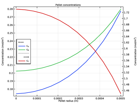
In the Model Builder window, expand the Results>Pellet Concentration at (0[m], 0[m], 0[m]) (tds) node, then click Pellet Concentration at (0[m], 0[m], 0[m]) (tds).
2
In the Settings window for 1D Plot Group, type Pellet Concentration at (0.5[m], 0[m], 0[m]) in the Label text field.
3
Locate the Data section. From the Time selection list, choose Last.
4
Click to expand the Title section. In the Title text area, type Pellet concentrations.
5
Locate the Plot Settings section. Select the Two y-axes check box.
6
In the table, select the Plot on secondary y-axis check box for Species C.
7
Locate the Legend section. From the Position list, choose Middle left.
Species A
1
In the Model Builder window, expand the Pellet Concentration at (0.5[m], 0[m], 0[m]) node, then click Species A.
2
In the Settings window for Line Graph, locate the y-Axis Data section.
3
In the Expression text field, type atxd3(0.5[m], 0[m], 0[m], tds.cpe_cA).
The syntax atxd3(0.5[m], 0[m], 0[m], comp1.tds.cpe_cA) means that you visualize the internal pellet concentration in a point 0.5 m from the inlet in the center of the column.
4
Click to expand the Coloring and Style section. From the Width list, choose 2.
5
Click to expand the Legends section. Find the Prefix and suffix subsection. In the Prefix text field, type c<sub>A</sub>.
Species B
1
In the Model Builder window, click Species B.
2
In the Settings window for Line Graph, locate the y-Axis Data section.
3
In the Expression text field, type atxd3(0.5[m], 0[m], 0[m], tds.cpe_cB).
4
Locate the Coloring and Style section. From the Width list, choose 2.
5
Locate the Legends section. Find the Prefix and suffix subsection. In the Prefix text field, type c<sub>B</sub>.
Species C
1
In the Model Builder window, click Species C.
2
In the Settings window for Line Graph, locate the y-Axis Data section.
3
In the Expression text field, type atxd3(0.5[m], 0[m], 0[m], tds.cpe_cC).
4
Locate the Coloring and Style section. From the Width list, choose 2.
5
Locate the Legends section. Find the Prefix and suffix subsection. In the Prefix text field, type c<sub>C</sub>.
6
In the Pellet Concentration at (0.5[m], 0[m], 0[m]) toolbar, click  Plot.
Pellet concentration, A
1
Click the  Zoom Extents button in the Graphics toolbar.
2
In the Model Builder window, under Results click Pellet concentration, A.
3
In the Pellet concentration, A toolbar, click  Plot.
Pellet concentration, A 1
Right-click Pellet concentration, A and choose Duplicate.
Pellets 1
1
In the Model Builder window, expand the Pellet concentration, A 1 node, then click Pellets 1.
2
In the Settings window for Pellets, locate the Data section.
3
From the Solution parameters list, choose From parent.
4
Locate the Coloring and Style section.
5
Select the Radius scale factor check box. In the associated text field, type 15.
Pellet and Bed Concentration, A
1
In the Model Builder window, under Results click Pellet concentration, A 1.
2
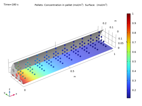
In the Settings window for 3D Plot Group, type Pellet and Bed Concentration, A in the Label text field.
3
Locate the Plot Settings section. Clear the Plot dataset edges check box.
Surface 1
Right-click Pellet and Bed Concentration, A and choose Surface.
Selection 1
1
In the Model Builder window, right-click Surface 1 and choose Selection.
2
Surface 1
1
In the Model Builder window, click Surface 1.
2
In the Settings window for Surface, click to expand the Inherit Style section.
3
From the Plot list, choose Pellets 1.
Surface: Outer Wall
1
In the Model Builder window, right-click Pellet and Bed Concentration, A and choose Surface.
2
In the Settings window for Surface, type Surface: Outer Wall in the Label text field.
3
Locate the Expression section. In the Expression text field, type 1.
4
Click to expand the Title section. From the Title type list, choose None.
5
Locate the Coloring and Style section. From the Coloring list, choose Uniform.
6
From the Color list, choose Gray.
Selection 1
1
Right-click Surface: Outer Wall and choose Selection.
2
3
In the Pellet and Bed Concentration, A toolbar, click  Plot.
Pellet and Bed Concentration, A
1
In the Model Builder window, click Pellet and Bed Concentration, A.
2
Drag and drop below Pellet concentration, C.
Next plot is created to visualize the difference in species’ average concentrations in the pellets and the reactor bed in the same plot. The figure requires a new dataset.
Cut Line 3D 1
In the Results toolbar, click  Cut Line 3D.
Concentration comparison
1
In the Results toolbar, click  1D Plot Group.
2
In the Settings window for 1D Plot Group, type Concentration comparison in the Label text field.
3
Locate the Data section. From the Dataset list, choose Cut Line 3D 1.
4
From the Time selection list, choose Last.
5
Locate the Title section. From the Title type list, choose Manual.
6
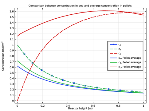
In the Title text area, type Comparison between concentration in bed and average concentration in pellets.
7
Locate the Plot Settings section.
8
Select the x-axis label check box. In the associated text field, type Reactor height (m).
9
Select the y-axis label check box. In the associated text field, type Concentration (mol/m<sup>3</sup>).
10
Locate the Legend section. From the Position list, choose Middle right.
A, bed
1
Right-click Concentration comparison and choose Line Graph.
2
In the Settings window for Line Graph, type A, bed in the Label text field.
3
Locate the Coloring and Style section. Find the Line style subsection. From the Line list, choose Dashed.
4
From the Width list, choose 2.
5
Find the Line markers subsection. From the Marker list, choose Point.
6
From the Positioning list, choose Interpolated.
7
In the Number text field, type 11.
8
Locate the Legends section. Select the Show legends check box.
9
From the Legends list, choose Manual.
10
B, bed
1
Right-click A, bed and choose Duplicate.
2
In the Settings window for Line Graph, type B, bed in the Label text field.
3
Locate the y-Axis Data section. In the Expression text field, type cB.
4
Locate the Coloring and Style section. Find the Line markers subsection. From the Marker list, choose None.
5
Locate the Legends section. In the table, enter the following settings:
C, bed
1
Right-click B, bed and choose Duplicate.
2
In the Settings window for Line Graph, type C, bed in the Label text field.
3
Locate the y-Axis Data section. In the Expression text field, type cC.
4
Locate the Legends section. In the table, enter the following settings:
A, pellet
1
Right-click C, bed and choose Duplicate.
2
In the Settings window for Line Graph, type A, pellet in the Label text field.
3
Locate the y-Axis Data section. In the Expression text field, type tds.pb1.pts1.avecpe_cA.
4
Locate the Coloring and Style section. Find the Line style subsection. From the Line list, choose Solid.
5
From the Color list, choose Cycle (reset).
6
Locate the Legends section. In the table, enter the following settings:
B, pellet
1
Right-click A, pellet and choose Duplicate.
2
In the Settings window for Line Graph, type B, pellet in the Label text field.
3
Locate the y-Axis Data section. In the Expression text field, type tds.pb1.pts1.avecpe_cB.
4
Locate the Coloring and Style section. From the Color list, choose Cycle.
5
Locate the Legends section. In the table, enter the following settings:
C, pellet
1
Right-click B, pellet and choose Duplicate.
2
In the Settings window for Line Graph, type C, pellet in the Label text field.
3
Locate the y-Axis Data section. In the Expression text field, type tds.pb1.pts1.avecpe_cC.
4
Locate the Legends section. In the table, enter the following settings:
5
In the Concentration comparison toolbar, click  Plot.
6
Click the  Zoom Extents button in the Graphics toolbar.
Bed Concentration, A, Streamline (tds)
Modify the default streamline plot. For high plot performance it is good to make them start on a cut plane above the bottom.
1
In the Model Builder window, under Results click Bed Concentration, A, Streamline (tds).
2
In the Settings window for 3D Plot Group, locate the Data section.
3
From the Dataset list, choose Sector 3D 1.
4
Locate the Plot Settings section. From the View list, choose Column view.
Cut Plane 1
1
In the Model Builder window, expand the Bed Concentration, A, Streamline (tds) node.
2
Right-click Results>Datasets and choose Cut Plane.
3
In the Settings window for Cut Plane, locate the Data section.
4
From the Dataset list, choose Sector 3D 1.
5
Locate the Plane Data section. In the X-coordinate text field, type 0.005.
Streamline 1
1
In the Model Builder window, under Results>Bed Concentration, A, Streamline (tds) click Streamline 1.
2
In the Settings window for Streamline, locate the Streamline Positioning section.
3
In the Points text field, type 1000.
4
From the Along curve or surface list, choose Cut Plane 1.
5
Locate the Coloring and Style section. Find the Line style subsection. From the Type list, choose Tube.
6
In the Tube radius expression text field, type cA[m^4/mol].
7
Select the Radius scale factor check box. In the associated text field, type .004.
You can zoom in by pressing down the middle mouse button and moving the mouse forward. Hold down the Ctrl-button to dolly in the camera position.
8
In the Bed Concentration, A, Streamline (tds) toolbar, click  Plot.
9
Click the  Zoom Extents button in the Graphics toolbar.
 
Appendix — Geometry Modeling Instructions
From the File menu, choose New.
New
In the New window, click  Model Wizard.
Model Wizard
1
In the Model Wizard window, click  3D.
2
Geometry 1
Work Plane 1 (wp1)
1
In the Geometry toolbar, click  Work Plane.
2
In the Settings window for Work Plane, locate the Plane Definition section.
3
From the Plane list, choose yz-plane.
4
Locate the Selections of Resulting Entities section. Find the Cumulative selection subsection. Click New.
5
In the New Cumulative Selection dialog box, type Inlet in the Name text field.
6
7
In the Settings window for Work Plane, click  Show Work Plane.
Work Plane 1 (wp1)>Circle 1 (c1)
1
In the Work Plane toolbar, click  Circle.
2
In the Settings window for Circle, locate the Size and Shape section.
3
In the Radius text field, type 0.017.
4
In the Sector angle text field, type 45.
5
Click  Build Selected.
Work Plane 1 (wp1)>Circle 2 (c2)
1
Right-click Component 1 (comp1)>Geometry 1>Work Plane 1 (wp1)>Plane Geometry>Circle 1 (c1) and choose Duplicate.
2
In the Settings window for Circle, locate the Size and Shape section.
3
In the Sector angle text field, type 180.
4
Locate the Position section. In the xw text field, type 0.017*2+0.02.
Work Plane 1 (wp1)>Circle 3 (c3)
1
Right-click Component 1 (comp1)>Geometry 1>Work Plane 1 (wp1)>Plane Geometry>Circle 2 (c2) and choose Duplicate.
2
In the Settings window for Circle, locate the Position section.
3
In the xw text field, type 0.017*4+0.02*2.
Work Plane 1 (wp1)>Circle 4 (c4)
1
Right-click Component 1 (comp1)>Geometry 1>Work Plane 1 (wp1)>Plane Geometry>Circle 3 (c3) and choose Duplicate.
2
In the Settings window for Circle, locate the Position section.
3
In the xw text field, type 0.017*6+0.02*3.
Work Plane 1 (wp1)>Circle 5 (c5)
1
Right-click Component 1 (comp1)>Geometry 1>Work Plane 1 (wp1)>Plane Geometry>Circle 4 (c4) and choose Duplicate.
2
In the Settings window for Circle, locate the Position section.
3
In the xw text field, type 0.017*2+0.02.
4
Locate the Rotation Angle section. In the Rotation text field, type 180.
Work Plane 1 (wp1)>Circle 6 (c6)
1
Right-click Component 1 (comp1)>Geometry 1>Work Plane 1 (wp1)>Plane Geometry>Circle 5 (c5) and choose Duplicate.
2
In the Settings window for Circle, locate the Position section.
3
In the xw text field, type 0.017*4+0.02*2.
Work Plane 1 (wp1)>Circle 7 (c7)
1
Right-click Component 1 (comp1)>Geometry 1>Work Plane 1 (wp1)>Plane Geometry>Circle 6 (c6) and choose Duplicate.
2
In the Settings window for Circle, locate the Position section.
3
In the xw text field, type 0.017*6+0.02*3.
4
In the Work Plane toolbar, click  Build All.
5
Click the  Zoom Extents button in the Graphics toolbar.
Work Plane 1 (wp1)>Rotate 1 (rot1)
1
In the Work Plane toolbar, click  Transforms and choose Rotate.
2
Select the objects c5, c6, and c7 only.
3
In the Settings window for Rotate, locate the Rotation section.
4
In the Angle text field, type 45.
5
Click  Build Selected.
Work Plane 1 (wp1)>Circle 8 (c8)
1
In the Model Builder window, under Component 1 (comp1)>Geometry 1>Work Plane 1 (wp1)>Plane Geometry right-click Circle 7 (c7) and choose Duplicate.
2
In the Settings window for Circle, locate the Size and Shape section.
3
In the Sector angle text field, type 360.
4
Locate the Position section. In the xw text field, type 0.017*4+0.02*2.
5
Locate the Rotation Angle section. In the Rotation text field, type 0.
6
Click  Build Selected.
Work Plane 1 (wp1)>Circle 9 (c9)
1
Right-click Component 1 (comp1)>Geometry 1>Work Plane 1 (wp1)>Plane Geometry>Circle 8 (c8) and choose Duplicate.
2
In the Settings window for Circle, locate the Position section.
3
In the xw text field, type 0.017*6+0.02*3.
4
Click  Build Selected.
Work Plane 1 (wp1)>Rotate 2 (rot2)
1
In the Work Plane toolbar, click  Transforms and choose Rotate.
2
Select the objects c8 and c9 only.
3
In the Settings window for Rotate, locate the Rotation section.
4
In the Angle text field, type 22.5.
5
Click  Build Selected.
Work Plane 2 (wp2)
1
In the Model Builder window, right-click Geometry 1 and choose Work Plane.
2
In the Settings window for Work Plane, locate the Plane Definition section.
3
From the Plane list, choose yz-plane.
4
Locate the Selections of Resulting Entities section. Find the Cumulative selection subsection. Click New.
5
In the New Cumulative Selection dialog box, type Bottom plate in the Name text field.
6
Work Plane 2 (wp2)>Plane Geometry
In the Model Builder window, click Plane Geometry.
Work Plane 2 (wp2)>Circle 1 (c1)
1
In the Work Plane toolbar, click  Circle.
2
In the Settings window for Circle, locate the Size and Shape section.
3
In the Radius text field, type .2.
4
In the Sector angle text field, type 45.
5
Click  Build Selected.
Extrude 1 (ext1)
1
In the Model Builder window, right-click Geometry 1 and choose Extrude.
2
In the Settings window for Extrude, click  Build Selected.
3
Click the  Zoom Extents button in the Graphics toolbar.
4
In the Geometry toolbar, click  Build All.
Create the last two selections.
5
In the Model Builder window, click Extrude 1 (ext1).
6
In the Settings window for Extrude, click  Build Selected.
Symmetry planes
1
In the Geometry toolbar, click  Selections and choose Explicit Selection.
2
In the Settings window for Explicit Selection, locate the Entities to Select section.
3
From the Geometric entity level list, choose Boundary.
4
On the object ext1, select Boundaries 2 and 3 only.
5
In the Label text field, type Symmetry planes.
Create the Outlet selection.
Outlet
1
Right-click Symmetry planes and choose Duplicate.
2
In the Settings window for Explicit Selection, type Outlet in the Label text field.
3
Locate the Entities to Select section. Find the Entities to select subsection. Click to select the  Activate Selection toggle button.
4
In the tree, select ext1>2 and ext1>3.
5
Click  Remove from Selection.
6
On the object ext1, select Boundary 5 only.
7
Click  Build All Objects.