PDF

Thermal Stresses in a Monolithic Reactor
Introduction
The removal of pollutants from high-temperature gases is often required in combustion processes. In this example, the selective reduction of NOx by ammonia occurs as flue gas passes through the channels of a monolithic reactor. The chemical reactions take place on a V2O5/TiO2 catalyst. The full reactor is a modular structure made up of blocks of reactive channels and supporting solid walls.
Figure 1: NOx reduction chemistry takes place in the channel blocks. Supporting walls hold together the full reactor geometry. Symmetry reduces the modeling domain to one eighth of the full reactor geometry.
Thermal gradients occur in the unit as heat is released by the chemical reactions while at the same time, heat is lost to the surroundings. This example investigates the thermal stresses in the reactor induced by the varying temperature field and the different material properties in the modular structure.
Note: This application requires the Chemical Reaction Engineering Module and the Structural Mechanics Module.
Model Definition
A separate model, NOx Reduction in a Monolithic Reactor, solves the coupled mass transport, heat transfer, and fluid flow equations representing the NOx reduction process in the reactor. Load this example from the Chemical Reaction Engineering Module Application Libraries and extend it by coupling the temperature field to a structural mechanics analysis to evaluate the thermal stresses in the reactor. For a more detailed description of the reaction kinetics, see Analysis of NOx Reaction Kinetics.
The Solid Mechanics interface has the equations and features required for stress analysis and general linear and nonlinear solid mechanics, solving for the structural displacements. Thermal loads are introduced into the constitutive equations according to:
where σ is the stress, D is the elasticity matrix, and ε represents the strain. The equation for the thermal strain is given by:
where α is the coefficient of thermal expansion, T is the temperature (K), and Tref is the strain-free reference temperature (K).
Reactor Materials
As mentioned above, the reactor treated in this example has a modular structure and is made up of blocks of reactive channels and supporting solid walls. Both materials are treated as being linear elastic. The wall material is isotropic while the channel block material is orthotropic. Their properties are summarized in the tables below:
νx = 0.19
νy = 0.021
νz = 0.021
Results and Discussion
Figure 2 shows the x-component of the stress tensor plotted in a number of cross sections. The highest negative values are found in the channel blocks closest to the center, signaling compressive stresses in this part of the reactor. This is a direct result of the temperature field in the reactor as shown in NOx Reduction in a Monolithic Reactor; the material in regions with high temperatures expand more than material at lower temperatures. The opposite effect is observed in channel blocks located near the outer surface of the reactor. In this relatively cold region the monolith structure experiences tensile stresses. The maximum compressive stress is evaluated to approximately 7.0 MPa and the maximum tensile stress is approximately 9.0 MPa. This indicates moderate stress levels in the monolith working under the stationary conditions presented in this example. More pronounced stress levels are expected as thermal gradients increase, for instance, during system startup.
Figure 2: The stress tensor component in the x direction. Compressive stress is indicated by negative values, and tensile stress by positive values.
Reference
1. G. Schaub, D. Unruh, J. Wang, and T. Turek, “Kinetic analysis of selective catalytic NOx reduction (SCR) in a catalytic filter,” Chem. Eng. and Processing, vol. 42, no. 5, pp. 365–371, 2003.
Application Library path: Chemical_Reaction_Engineering_Module/Reactors_with_Porous_Catalysts/monolith_thermal_stress
Modeling Instructions
Application Libraries
1
From the File menu, choose Application Libraries.
2
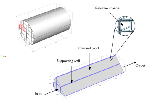
In the Application Libraries window, select Chemical Reaction Engineering Module>Tutorials>monolith_3d in the tree.
3
3D Model (comp2)
Add a Solid Mechanics interface to extend the model with an analysis of the thermal stresses in the reactor materials.
Add Physics
1
In the Home toolbar, click  Add Physics to open the Add Physics window.
2
Go to the Add Physics window.
3
In the tree, select Structural Mechanics>Solid Mechanics (solid).
4
Find the Physics interfaces in study subsection. In the table, clear the Solve check boxes for Study 1 and Study 2.
5
Click Add to 3D Model in the window toolbar.
Add Study
1
In the Home toolbar, click  Add Study to open the Add Study window.
2
Go to the Add Study window.
3
Find the Studies subsection. In the Select Study tree, select Preset Studies for Some Physics Interfaces>Stationary.
4
Click Add Study in the window toolbar.
5
In the Home toolbar, click  Add Study to close the Add Study window.
Study 3
Step 1: Stationary
1
In the Home toolbar, click  Add Physics to close the Add Physics window.
2
Click the  Zoom Extents button in the Graphics toolbar.
Solid Mechanics (solid)
Two Linear Elastic Material models are needed for the analysis, one for the supporting wall material and one for the channel blocks. Note that the wall material is isotropic while the block material is orthotropic.
Linear Elastic Material 2
1
In the Model Builder window, under 3D Model (comp2) right-click Solid Mechanics (solid) and choose Material Models>Linear Elastic Material.
2
In the Settings window for Linear Elastic Material, locate the Domain Selection section.
3
From the Selection list, choose Supporting walls.
4
Locate the Linear Elastic Material section. From the E list, choose User defined. In the associated text field, type 1.5e9.
5
From the ν list, choose User defined. In the associated text field, type 0.2.
Add a Thermal Expansion feature to each Linear Elastic node. The features receive the temperature field solved by the Heat Transfer in Fluids interface as Model Input.
Thermal Expansion 1
1
In the Physics toolbar, click  Attributes and choose Thermal Expansion.
2
In the Settings window for Thermal Expansion, locate the Thermal Expansion Properties section.
3
From the α list, choose User defined. In the associated text field, type 2.7e-6.
Linear Elastic Material 1
1
In the Model Builder window, under 3D Model (comp2)>Solid Mechanics (solid) click Linear Elastic Material 1.
2
In the Settings window for Linear Elastic Material, locate the Linear Elastic Material section.
3
From the Material symmetry list, choose Orthotropic.
4
From the E list, choose User defined. Specify the associated vector as
5
From the ν list, choose User defined. Specify the associated vector as
6
From the G list, choose User defined. Specify the associated vector as
Thermal Expansion 1
1
In the Physics toolbar, click  Attributes and choose Thermal Expansion.
2
In the Settings window for Thermal Expansion, locate the Thermal Expansion Properties section.
3
From the α list, choose User defined. In the associated text field, type 4e-6.
Complete the setup of the structural mechanics problem by defining the following boundary conditions.
Roller 1
1
In the Physics toolbar, click  Boundaries and choose Roller.
2
You can use the Selection List from the View menu.
Symmetry 1
1
In the Physics toolbar, click  Boundaries and choose Symmetry.
2
In the Settings window for Symmetry, locate the Boundary Selection section.
3
From the Selection list, choose Symmetry.
Follow the steps below to solve only the structural mechanics problem, using the temperature field from the solved reactor model as input to the calculations.
Study 3
1
In the Model Builder window, click Study 3.
2
In the Settings window for Study, locate the Study Settings section.
3
Clear the Generate default plots check box.
This selection turns off the plots set up by default for each of the physics interfaces.
Step 1: Stationary
Clear all physics interfaces except Solid Mechanics to solve only for the displacement field.
1
In the Model Builder window, under Study 3 click Step 1: Stationary.
2
In the Settings window for Stationary, locate the Physics and Variables Selection section.
3
In the table, clear the Solve for check boxes for Reaction Engineering (re), Chemistry 1 (chem), Transport of Diluted Species in Porous Media (tds), Heat Transfer in Porous Media 1 (ht), and Darcy’s Law 1 (dl).
Now, instruct the solver to use the results from the monolith 3D model for the variables not solved for.
4
Click to expand the Values of Dependent Variables section. Find the Values of variables not solved for subsection. From the Settings list, choose User controlled.
5
From the Method list, choose Solution.
6
From the Study list, choose Study 2, Stationary.
The monolith 3D model results are stored under Study 2.
7
In the Home toolbar, click  Compute.
Results
The Datasets node allows you great freedom to define tailored sets of plot data to be used by the plot nodes. Here, use the Mirror 3D feature to reflect the results in the symmetry planes of the model.
Mirror the data in the symmetry plane that is at a 45 degree angle to the xy-plane.
Mirror 3D 1
1
In the Results toolbar, click  More Datasets and choose Mirror 3D.
2
In the Settings window for Mirror 3D, locate the Data section.
3
From the Dataset list, choose Study 3/Solution 37 (sol37).
4
Locate the Plane Data section. From the Plane type list, choose General.
5
In row Point 2, set X to 0.1.
6
In row Point 3, set Y to 3.575e-3 and Z to 3.575e-3.
Thermal Stress
1
In the Results toolbar, click  3D Plot Group.
2
In the Settings window for 3D Plot Group, type Thermal Stress in the Label text field.
3
Locate the Data section. From the Dataset list, choose Mirror 3D 1.
4
Click to expand the Title section. From the Title type list, choose None.
5
Locate the Color Legend section. Select the Show units check box.
Slice 1
1
Right-click Thermal Stress and choose Slice.
2
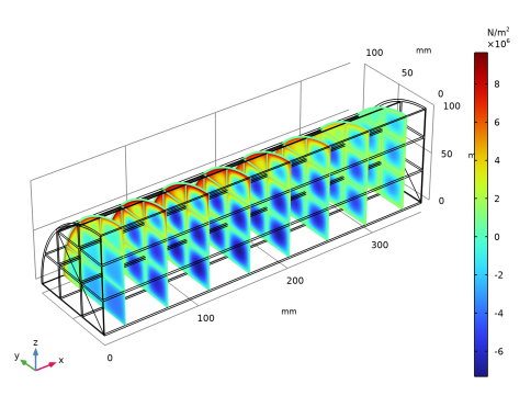
In the Settings window for Slice, click Replace Expression in the upper-right corner of the Expression section. From the menu, choose 3D Model (comp2)>Solid Mechanics>Stress>Stress tensor (spatial frame) - N/m²>solid.sxx - Stress tensor, xx-component.
3
Locate the Plane Data section. In the Planes text field, type 8.
4
In the Thermal Stress toolbar, click  Plot.
5
Click the  Zoom Extents button in the Graphics toolbar.