You are viewing the documentation for an older COMSOL version. The latest version is available here.
PDF

Gold Recycling Through Oxidative Dissolution
Introduction
Recovery of precious metals in recycling of electronics, or extraction from ore, is usually performed through leaching of the metal into an aqueous phase. Precious metals require the use of an oxidant and, often, a complexant. In the case of gold, the cyanide anion CN- forms a soluble complex with gold(I) (that is, Au(CN)-2), that is so stable that molecular oxygen becomes a viable oxidant. The process is known as gold cyanidation, and it has — unsurprisingly — been studied extensively for the past century. Research into finding less toxic complexants is ongoing, but due to the availability of kinetic parameters, this model sticks to using cyanide.
The model studies the oxidative dissolution of this noble metal in an air saturated cyanide solution. The system encompasses three phases: a gaseous phase (air), an aqueous phase, and a solid gold phase. The system is assumed to be homogeneous on a macroscopic scale, for example fine particulate matter dispersed in water, which is continuously agitated by a stream of air bubbles.
Model Definition
Since this problem is not limited by mass transport in the bulk, it will be modeled in a 0D component. The rate limiting step is that of a surface reaction, and corresponds to a problem where diffusion is not a rate limiting step, which is in line with a recent model. Since the evolution of available surface area during dissolution depends on the geometry of the particles, the model includes two cases: flakes and spheres (see Figure 1), each in its separate 0D component.
Figure 1: The two cases studied, flakes (to the left) and spheres (to the right).
Liquid phase
In each component, two Reaction Engineering interfaces will be added, the first one will describe the liquid phase, in which the following reaction is added:
The rate of reaction is, according to Ref. 1:
(1)
where A is total exposed surface area of gold, V is the volume of the liquid, kAu is a parameterized rate constant, and c' is the product between the adsorption coefficient of cyanide on gold (Kads), the concentration of aqueous dioxygen, and the concentration of cyanide to the power of three:
(2)
Assume that the starting material is monodisperse; that is, that all particles are of the same size. The total amount of gold per unit of volume (the so called loading) is set equal in the two components, and the thickness of the flakes is set such that initial surface areas of the two cases are equal. Since the system is assumed to be well mixed, the concentration of oxygen is set to be in equilibrium with the partial pressure in the gas phase.
Gas Phase
The second Reaction Engineering interface will represent the gas phase (air). Add two species: O2 and N2, but only the former will participate in any reactions. A global constraint, requiring Henry’s Law for O2 to be fulfilled at all times, is added, and since the system is considered to be a batch reactor (where oxygen can be depleted), introduce an additional constraint, enforcing mass conservation of the total amount of oxygen.
Differences Between the Components
In the first component, the dissolution of flakes is modeled. Here assume that the total surface area exposed remains constant throughout the reaction (the flakes are assumed to be utterly oblate) up to the point that the last bit of solid has been consumed, at which point the available surface area is assumed to drop to zero. In order not to introduce a discontinuity in the available surface area, assign a smoothed stepping function which rapidly falls around the point at which depletion occurs.
In the second component, describing dissolution of spheres, the surface area exposed does vary during the course of the dissolution process (the surface area is proportional to the mass loading of gold to the power of two thirds). Since the surface area naturally goes to zero as the amount of solid gold declines, it is possible to do away with the smoothed stepping function, but as the solver approaches the end of the reaction, care is taken to avoid evaluating the fractional power of a negative number.
Results and Discussion
The result of the time integration is shown in Figure 2.
Figure 2: Time evolution of concentrations and partial pressure of oxygen for each of the two particle cases.
The initial conditions are the same for both studies, and also the initial rates of change are the same for the two components. But as the spheres dissolve, their total surface area decreases, leading to a slower leaching compared to the flakes. After some time the leaching process in the system with flakes stops runs out of solid gold and all reactions stop, whereas this quantity in the system with spherical particles is still asymptotically approaching zero.
Reference
1. G. Senanayake, “Kinetics and reaction mechanism of gold cyanidation: Surface reaction model via Au(I)–OH–CN complexes,” Hydrometallurgy, vol. 80, pp. 1–12, 2005.
Application Library path: Chemical_Reaction_Engineering_Module/Ideal_Tank_Reactors/gold_recycling
Modeling Instructions
From the File menu, choose New.
New
In the New window, click  Model Wizard.
Model Wizard
1
In the Model Wizard window, click  0D.
2
In the Select Physics tree, select Chemical Species Transport>Reaction Engineering (re).
3
4
Click  Study.
5
In the Select Study tree, select General Studies>Time Dependent.
6
Liquid phase
Add a Reaction Engineering interface, which will correspond to the liquid phase.
1
In the Model Builder window, under Component 1 (comp1) click Reaction Engineering (re).
2
In the Settings window for Reaction Engineering, type Liquid phase in the Label text field.
3
Locate the Reactor section. Find the Mass balance subsection. In the Vr text field, type V_liquid.
4
Locate the Energy Balance section. In the T text field, type T.
5
Locate the Mixture Properties section. From the Phase list, choose Liquid.
Global Definitions
Parameters 1
Read in a set of parameters to be used in the model (V_liquid being one of them).
1
In the Model Builder window, under Global Definitions click Parameters 1.
2
In the Settings window for Parameters, locate the Parameters section.
3
Click  Load from File.
4
The first component describes a system with dispersed gold flakes dissolving in a liquid, while maintaining a constant interfacial area to the liquid phase. Read in variables describing this behavior into the variables section of Component 1.
Definitions
Variables 1
1
In the Model Builder window, under Component 1 (comp1) right-click Definitions and choose Variables.
2
In the Settings window for Variables, locate the Variables section.
3
Click  Load from File.
4
Liquid phase (re)
Define a reaction describing the overall dissolution process, where gold is oxidized by molecular oxygen into a gold(I)dicyanide complex.
Reaction 1
1
In the Reaction Engineering toolbar, click  Reaction.
2
In the Settings window for Reaction, locate the Reaction Formula section.
3
In the Formula text field, type Au(s) + CN- + O2(aq) + H2O => AuCNCN- + OH-.
Use the Balance feature to determine the coefficients for the reactants and products.
4
Click Balance in the upper-right corner of the Reaction Formula section.
The effective rate expression does not follow the law of mass action, instead use the rate expression derived in the reference publication.
5
Locate the Reaction Rate section. From the list, choose User defined.
6
In the rj text field, type flakes_R_Au/4.
While not strictly needed, set the rate parameters to descriptive values.
7
Find the Volumetric overall reaction order subsection. In the Forward text field, type 4.
8
Locate the Rate Constants section. In the kf text field, type 0.
Initial Values 1
Enter initial values for a slightly alkaline (pH: 9.4) air saturated aqueous solution.
1
In the Model Builder window, click Initial Values 1.
2
In the Settings window for Initial Values, locate the Volumetric Species Initial Values section.
3
Dissolution of gold flakes
Enter a descriptive label for the first component, which treats the case of thin foil or flakes of gold.
1
In the Model Builder window, click Component 1 (comp1).
2
In the Settings window for Component, type Dissolution of gold flakes in the Label text field.
Add Physics
1
In the Reaction Engineering toolbar, click  Add Physics to open the Add Physics window.
2
Go to the Add Physics window.
Add a second Reaction Engineering interface corresponding to the gas phase.
3
In the tree, select Recently Used>Reaction Engineering (re).
4
Click Add to Dissolution of Gold Flakes in the window toolbar.
5
In the Reaction Engineering toolbar, click  Add Physics to close the Add Physics window.
Gas Phase
1
In the Settings window for Reaction Engineering, type Gas Phase in the Label text field.
The gas phase is compressible, hence its volume is not guaranteed to remain constant, change the reactor type to batch to reflect this fact.
2
Locate the Reactor section. From the Reactor type list, choose Batch.
The volume of the gas phase is defined as a variable depending on the total volume and the volume of the (assumed incompressible) liquid and solid phases.
3
Find the Mass balance subsection. In the Vr text field, type V_gas.
4
Locate the Energy Balance section. In the T text field, type T.
Oxygen will be present in both gas and liquid phase, next add it as a gas phase species.
Species 1
1
Right-click Dissolution of gold flakes (comp1)>Gas Phase and choose Species.
2
In the Settings window for Species, locate the Name section.
3
For completeness, also add nitrogen, even though it will not participate in any chemical reactions.
4
In the Reaction Engineering toolbar, click  Species.
Species 1
1
In the Settings window for Species, locate the Name section.
2
The concentration of oxygen in the gas phase and in the liquid phase, is assumed to equilibrate on a much shorter time scale than the chemical reaction consuming oxygen (for example, a well stirred system). Hence, at any given time, Henry’s law is assumed to be fulfilled. We can impose this by introducing a Global Constraint
3
Click the  Show More Options button in the Model Builder toolbar.
4
In the Show More Options dialog box, in the tree, select the check box for the node Physics>Equation-Based Contributions.
5
Henry’s Law for Dioxygen
1
In the Reaction Engineering toolbar, click  Global Constraint.
2
In the Settings window for Global Constraint, type Henry's Law for Dioxygen in the Label text field.
3
Locate the Global Constraint section. In the Constraint expression text field, type re.c_O2_aq - H_O2*R_const*T*re2.c_O2_gas.
Since Henry’s law only dictates that the ratio of concentrations needs to remain constant, the solver would be free to, for example, increase both concentrations, but with different amounts. Clearly this would violate mass conservation. Therefore, add a second constraint on the total amount of oxygen atoms in our system.
Mass Conservation of Oxygen
1
In the Reaction Engineering toolbar, click  Global Constraint.
2
In the Settings window for Global Constraint, type Mass Conservation of Oxygen in the Label text field.
3
Locate the Global Constraint section. In the Constraint expression text field, type V0_gas*(2*re2.c_O2_gas - 2*re2.c0_O2_gas) + V_liquid*(2*re.c_O2_aq + re.c_H2O + re.c_OH_1m - 2*re.c0_O2_aq - re.c0_H2O - re.c0_OH_1m).
Initial Values 1
The model starts with air.
1
In the Model Builder window, click Initial Values 1.
2
In the Settings window for Initial Values, locate the Volumetric Species Initial Values section.
3
Currently the rate of reaction is assumed independent of the amount of gold in our system. This corresponds to a constant area of gold interface during the dissolution, which is a good assumption for flakes or foil. However, once the gold is consumed, the reaction will need to stop, or else we would obtain negative concentrations of gold. Therefore we will modulate our rate of reaction with a step function, essentially a smoothed version of Heaviside’s step function.
Global Definitions
Step 1 (step1)
1
In the Home toolbar, click  Functions and choose Global>Step.
2
In the Settings window for Step, click  Plot.
3
Locate the Parameters section. In the From text field, type -1.
4
This function, step1 is already being referred to in the Variables 1 section.
Dissolution of gold flakes (comp1)
Copy the first component for modeling flakes of gold, and create a second component for a (spherical) particulate suspension.
1
In the Model Builder window, right-click Dissolution of gold flakes (comp1) and choose Copy.
Dissolution of spherical gold
1
In the Model Builder window, right-click the root node and choose Paste Multiple Items.
Give the component a descriptive label.
2
In the Settings window for Component, type Dissolution of spherical gold in the Label text field.
Definitions (comp2)
Variables 1
In the interest of minimizing the amount of manual input, load variable expressions from a file.
1
In the Model Builder window, under Dissolution of spherical gold (comp2)>Definitions click Variables 1.
2
In the Settings window for Variables, locate the Variables section.
3
Click  Clear Table.
4
Click  Load from File.
5
Note how the rate of gold dissolution depends on remaining surface area, because of that, this formulation does not need a step function.
Liquid phase (re3)
1: 4Au(s)+8CN-+O2(aq)+2H2O=>4AuCNCN-+4OH-
Update the rate expression to refer to this spherical case.
1
In the Model Builder window, expand the Dissolution of spherical gold (comp2)>Liquid phase (re3) node, then click 1: 4Au(s)+8CN-+O2(aq)+2H2O=>4AuCNCN-+4OH-.
2
In the Settings window for Reaction, locate the Reaction Rate section.
3
In the rj text field, type spherical_R_Au/4.
Gas Phase (re4)
Henry’s Law for Dioxygen
Update the qualified names so that they refer to the interfaces in our new component.
1
In the Model Builder window, expand the Dissolution of spherical gold (comp2)>Gas Phase (re4) node, then click Henry’s Law for Dioxygen.
2
In the Settings window for Global Constraint, locate the Global Constraint section.
3
In the Constraint expression text field, type re3.c_O2_aq - H_O2*R_const*T*re4.c_O2_gas.
Mass Conservation of Oxygen
1
In the Model Builder window, click Mass Conservation of Oxygen.
2
In the Settings window for Global Constraint, locate the Global Constraint section.
3
In the Constraint expression text field, type V0_gas*(2*re4.c_O2_gas - 2*re4.c0_O2_gas) + V_liquid*(2*re3.c_O2_aq + re3.c_H2O + re3.c_OH_1m - 2*re3.c0_O2_aq - re3.c0_H2O - re3.c0_OH_1m).
At this point the model is ready for solving, solve for 15 h.
Study 1
Step 1: Time Dependent
1
In the Model Builder window, under Study 1 click Step 1: Time Dependent.
2
In the Settings window for Time Dependent, locate the Study Settings section.
3
From the Time unit list, choose min.
4
In the Output times text field, type range(0,1,600).
5
In the Home toolbar, click  Compute.
Disable all but one plot group.
Results
Concentration (re2), Concentration (re3), Concentration (re4)
1
In the Model Builder window, under Results, Ctrl-click to select Concentration (re2), Concentration (re3), and Concentration (re4).
2
Load expressions for plotting from files.
Liquid (flakes)
1
In the Model Builder window, expand the Results>Concentration (re) node, then click Global 1.
2
In the Settings window for Global, type Liquid (flakes) in the Label text field.
3
Locate the y-Axis Data section. Click  Clear Table.
4
Click  Load from File.
5
6
Click to expand the Legends section. Find the Include subsection. Select the Description check box.
7
Clear the Expression check box.
Liquid (spheres)
1
In the Model Builder window, right-click Concentration (re) and choose Global.
2
In the Settings window for Global, type Liquid (spheres) in the Label text field.
3
Locate the y-Axis Data section. Click  Clear Table.
4
Click  Load from File.
5
6
Click to expand the Coloring and Style section. Find the Line style subsection. From the Line list, choose Dashed.
7
From the Color list, choose Cycle (reset).
8
Locate the Legends section. Find the Include subsection. Select the Description check box.
9
Clear the Expression check box.
Gas
1
Right-click Concentration (re) and choose Global.
2
In the Settings window for Global, type Gas in the Label text field.
3
Locate the y-Axis Data section. Click  Clear Table.
4
Click  Load from File.
5
6
Locate the Coloring and Style section. Find the Line style subsection. From the Line list, choose Cycle.
7
From the Color list, choose Black.
8
Locate the Legends section. Find the Include subsection. Select the Description check box.
9
Clear the Expression check box.
Concentration (re)
1
In the Model Builder window, click Concentration (re).
2
In the Settings window for 1D Plot Group, click to expand the Title section.
3
From the Title type list, choose Manual.
4
In the Title text area, type Aqueous Gold Dissolution of Flakes and Spheres.
5
Locate the Plot Settings section. Select the Two y-axes check box.
6
In the table, select the Plot on secondary y-axis check box for Gas.
7
Select the x-axis label check box. In the associated text field, type Time (min).
8
Select the y-axis label check box. In the associated text field, type Concentration (mM).
9
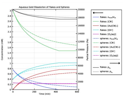
Select the Secondary y-axis label check box. In the associated text field, type Partial Pressure (Pa).
10
Locate the Axis section. Select the Manual axis limits check box.
11
In the y minimum text field, type 0.
12
In the Secondary y minimum text field, type 0.
13
In the x maximum text field, type 600.
14
Locate the Legend section. From the Layout list, choose Outside graph axis area.
15
In the Concentration (re) toolbar, click  Plot.
This is Figure 2.