You are viewing the documentation for an older COMSOL version. The latest version is available here.
PDF

Drug Release from a Biomaterial Matrix
Introduction
Biomaterial matrices for drug release are useful for in vivo tissue regeneration. The following example describes the release of a drug from a biomaterial matrix into damaged cell tissue. Specifically, a nerve guide delivers a regenerating drug to damaged nerve ends.
This model examines detailed drug-release kinetics, with rate expressions handling drug dissociation/association reactions as well as matrix degradation by enzyme catalysis. The enzyme reaction is described by Michaelis–Menten kinetics. The model enables investigation of design parameters governing the rate of drug release such as drug-to-biomaterial affinity, biomaterial degradation, drug loading, and the influence of geometry and composition of the biomaterial matrix.
Model Definition
The model consists of two parts. One part uses the batch reactor type in the Reaction Engineering interface to specify the reacting system in a perfectly mixed environment, that is, no space dependency is assumed. The purpose of this part is to study the reaction kinetics. The second part includes a space dependent component generated from the Reaction Engineering interface. It utilizes the Transport of Diluted Species in Porous Catalysts interface and serves to investigate the drug transport from the biomaterial into a region with damaged nerve ends.
Figure 1 shows the full 3D geometry as well as the 2D modeling domain, reduced by axial symmetry and a mirror plane, for the space-dependent model. The biomaterial holding the drug is assumed to have a strictly cylindrical shape. The three distinct areas (domains) are:
Figure 1: The full 3D geometry (left) and the equivalent modeling domains reduced to 2D by axial symmetry (right). The regions are: the nerve-cell tissue, the biomaterial matrix, and the surrounding medium.
In the biomaterial, a drug molecule, d, binds to a peptide, p, which in turn is anchored to the matrix, m. Matrix-bound species are labeled mpd and mp, respectively, the latter referring to a species where no drug is bound to the peptide. The species mpd and mp are modeled as surface species attached to the matrix surface, and are only present in the biomaterial.
Two mechanisms release the drug from the matrix. First, the drug can simply dissociate from the matrix site mp. Second, matrix degradation by an enzyme, e, originating from the cell-tissue domain, leads to release of the drug-peptide species, pd, from which the drug subsequently dissociates. The unbound species p, d, pd, and e are free bulk species and present in the entire model geometry. Figure 2 illustrates the complete reaction scheme.
Figure 2: Reaction scheme describing drug dissociation/association reactions (horizontal) and matrix-degradation reactions (vertical).
The time-dependent mass balance per species is described by
(1)
where Dik (SI unit: m2/s) is the diffusion coefficient for species i   in the respective medium k. In the right-hand side Rik (SI unit: mol/(m3·s)) is the rate expression for volumetric reactions, involving bulk species only, of species i  in domain k. The second term on the right-hand side results from surface reactions involving matrix-bound species (mpd and mp) in the biomaterial. Rs,i is the surface reaction rate (SI unit: mol/(m2·s)) and Ssa the specific surface area of the biomaterial (SI unit: 1/m).
In the biomaterial (index k = 2), all the reactions described in Figure 2 are possible, leading to the following rate expressions:
The rate terms RMMmp and RMMmpd  refer to the Michaelis–Menten kinetics describing the enzyme catalyzed degradation of the matrix:
with
RMMmp  describes the disappearance of mp sites and the production of p species. RMMmpd  describes the disappearance of mpd sites and the production of pd species. Vmax is the maximum rate and KM the Michaelis–Menten constant. In the cell region (index k = 1) and in the surrounding medium (index k = 3) only dissociation/association reactions occur, leading to the rate expressions
The boundary condition is axial symmetry along the rotational axis and insulation/symmetry elsewhere. Values for diffusion coefficients and rate constants come from the literature (Ref. 1).
Results and Discussion
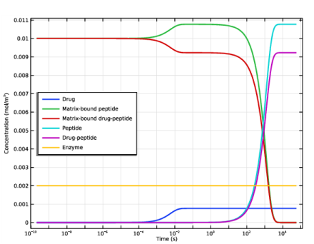
Figure 3 shows the concentration transients of the reacting species in a perfectly mixed (space-independent) system.
Figure 3: Concentrations of all reacting species (mol/m3) as functions of time (s).
The effect of enzyme degradation is clearly visible, with matrix-bound peptide species (mp and mpd) decreasing and free peptide species (p and pd) increasing with time. The matrix is completely degraded after approximately 5000 seconds. As the drug and peptide species have the same association/dissociation kinetics, no matter the peptide is free or matrix-bound, the steady-state concentration of drug is constant during the degradation process.
Solving the space-dependent mass balances of Equation 1 results in concentration distributions of all participating species as functions of time. Figure 4 shows the concentration of all bulk species.
Figure 4: Bulk species concentrations after 1.5 h.
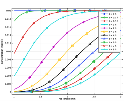
As mentioned earlier, the enzyme originates from the nerve-cell tissue. From Figure 5, where the total drug release is shown, it is clear that matrix degradation has a directing effect on the drug release toward the damaged cell region.
Figure 5: Concentration profiles describing the total drug concentration (cd + cpd) across the modeling domain.
Figure 6 visualizes the biomaterial matrix degradation. The plotted total matrix site concentrations (cmp + cmpd) shows how the degradation front passes through the biomaterial geometry.
Figure 6: Concentration profiles describing the total matrix site concentration (cmp + cmpd).
Figure 7 shows how the drug distribution in the different domains vary during the simulation. It can be noted that the drug level in the biomaterial reaches a maximum after about 5 hours. The same is true for the drug level in the nerve.
Figure 7: Drug distribution among the different domains.
The detailed reaction/transport description in this model allows for the investigation of many design parameters relevant to bioengineering. This case presents the effect of matrix degradation on drug release as a function of time and geometry. Furthermore, it is straightforward to study the influence of the drug/peptide affinity by varying the rate constants kf1 and kr1, or the influence of drug loading by varying the cmp : cmpd ratio. The ability to examine alternative geometries and mixed biomaterial domains gives even more design flexibility.
Reference
1. D.J. Maxwell, B.C. Hicks, S. Parsons, and S.E. Sakiyama-Elbert, “Development of rationally designed affinity-based drug delivery systems”, Acta Biomat., vol. 1, no. 1, pp. 101–113, 2005.
Application Library path: Chemical_Reaction_Engineering_Module/Reactors_with_Mass_Transfer/drug_release
Modeling Instructions
From the File menu, choose New.
New
In the New window, click  Model Wizard.
Model Wizard
1
In the Model Wizard window, click  0D.
2
In the Select Physics tree, select Chemical Species Transport>Reaction Engineering (re).
3
Click Add.
4
Click  Study.
5
In the Select Study tree, select General Studies>Time Dependent.
6
Reaction Engineering (re)
Read global parameters from a text file.
Global Definitions
Parameters 1
1
In the Model Builder window, under Global Definitions click Parameters 1.
2
In the Settings window for Parameters, locate the Parameters section.
3
Click  Load from File.
4
Reaction Engineering (re)
First, model the reaction behavior of drug release from the biomaterial matrix, regarding the material as a perfectly mixed batch reactor.
1
In the Model Builder window, under Component 1 (comp1) click Reaction Engineering (re).
2
In the Settings window for Reaction Engineering, locate the Mixture Properties section.
3
From the Phase list, choose Liquid.
Reaction 1
1
In the Reaction Engineering toolbar, click  Reaction.
2
In the Settings window for Reaction, locate the Reaction Formula section.
3
In the Formula text field, type d+mp(ads)=>mpd(ads).
4
Click Apply.
5
From the Reaction type list, choose Reversible.
6
Locate the Rate Constants section. In the kf text field, type kf_d.
7
In the kr text field, type kr_d.
Reaction 2
1
In the Reaction Engineering toolbar, click  Reaction.
2
In the Settings window for Reaction, locate the Reaction Formula section.
3
In the Formula text field, type d+p<=>pd.
4
Click Apply.
5
Locate the Rate Constants section. In the kf text field, type kf_d.
6
In the kr text field, type kr_d.
Reaction 3
1
In the Reaction Engineering toolbar, click  Reaction.
Add the reactions describing the enzyme catalyzed degradation of the matrix. mp and mpd sites are consumed while producing free p and d species.
2
In the Settings window for Reaction, locate the Reaction Formula section.
3
In the Formula text field, type mp(ads)+e=>p+e.
4
Click Apply.
5
Locate the Reaction Rate section. From the list, choose User defined.
6
In the rj text field, type kf_mm*re.c_e*re.csurf_mp_surf/(Km+re.csurf_mp_surf*Ssa).
Reaction 4
1
In the Reaction Engineering toolbar, click  Reaction.
2
In the Settings window for Reaction, locate the Reaction Formula section.
3
In the Formula text field, type mpd(ads)+e=>pd+e.
4
Click Apply.
5
Locate the Reaction Rate section. From the list, choose User defined.
6
In the rj text field, type kf_mm*re.c_e*re.csurf_mpd_surf/(Km+re.csurf_mpd_surf*Ssa).
Species 1
1
In the Reaction Engineering toolbar, click  Species.
2
In the Settings window for Species, locate the Name section.
3
4
Locate the Type section. From the list, choose Solvent.
5
In the Model Builder window, click Reaction Engineering (re).
6
In the Settings window for Reaction Engineering, locate the Reactor section.
7
Find the Surface reaction area subsection. Click the Surface area to volume ratio button.
8
In the as text field, type Ssa.
Initial Values 1
1
In the Model Builder window, click Initial Values 1.
2
In the Settings window for Initial Values, locate the Volumetric Species Initial Values section.
3
4
Locate the Surface Species Initial Values section. In the table, enter the following settings:
5
In the Γs text field, type (cmp_init+cmpd_init).
Study 1
Step 1: Time Dependent
1
In the Model Builder window, under Study 1 click Step 1: Time Dependent.
2
In the Settings window for Time Dependent, locate the Study Settings section.
3
From the Time unit list, choose h.
4
In the Output times text field, type range(0,0.1,16).
5
In the Home toolbar, click  Compute.
Results
Biomaterial Concentrations, 0D model
Follow these steps to create Figure 3.
1
In the Settings window for 1D Plot Group, type Biomaterial Concentrations, 0D model in the Label text field.
2
Click the  x-Axis Log Scale button in the Graphics toolbar.
Global 1
1
In the Model Builder window, expand the Biomaterial Concentrations, 0D model node, then click Global 1.
2
In the Settings window for Global, locate the y-Axis Data section.
3
4
Locate the x-Axis Data section. From the Unit list, choose s.
5
Click to expand the Coloring and Style section. From the Width list, choose 2.
6
In the Biomaterial Concentrations, 0D model toolbar, click  Plot.
7
Click to expand the Legends section. From the Legends list, choose Manual.
8
9
In the Biomaterial Concentrations, 0D model toolbar, click  Plot.
10
Click the  Zoom Extents button in the Graphics toolbar.
Biomaterial Concentrations, 0D model
1
In the Model Builder window, click Biomaterial Concentrations, 0D model.
2
In the Settings window for 1D Plot Group, click to expand the Title section.
3
From the Title type list, choose None.
4
Locate the Plot Settings section.
5
Select the y-axis label check box. In the associated text field, type Concentration (mol/m<sup>3</sup>).
6
Locate the Legend section. From the Position list, choose Middle left.
Start setting up the space-dependent model by exporting the settings of the Reaction Engineering interface with the Generate Space-Dependent Model feature.
Reaction Engineering (re)
Generate Space-Dependent Model 1
1
In the Reaction Engineering toolbar, click  Generate Space-Dependent Model.
2
In the Settings window for Generate Space-Dependent Model, locate the Component Settings section.
3
From the Component to use list, choose 2Daxi: New.
4
Locate the Physics Interfaces section. Find the Chemical species transport subsection. From the list, choose Transport of Diluted Species in Porous Catalysts: New.
5
Locate the Study Type section. From the Study type list, choose Time dependent.
6
Locate the Space-Dependent Model Generation section. Click Create/Refresh.
Component 2 (comp2)
In the Model Builder window, expand the Component 2 (comp2) node.
Geometry 1(2Daxi)
1
In the Model Builder window, expand the Component 2 (comp2)>Geometry 1(2Daxi) node, then click Geometry 1(2Daxi).
2
In the Settings window for Geometry, locate the Units section.
3
From the Length unit list, choose mm.
Rectangle 1 (r1)
1
In the Geometry toolbar, click  Rectangle.
2
In the Settings window for Rectangle, locate the Size and Shape section.
3
In the Width text field, type 6.
4
In the Height text field, type 9.
Rectangle 2 (r2)
1
Right-click Rectangle 1 (r1) and choose Duplicate.
2
In the Settings window for Rectangle, locate the Size and Shape section.
3
In the Width text field, type 1.
Rectangle 3 (r3)
1
Right-click Rectangle 2 (r2) and choose Duplicate.
2
In the Settings window for Rectangle, locate the Size and Shape section.
3
In the Width text field, type 2.
4
In the Height text field, type 6.
5
Locate the Position section. In the r text field, type 1.
6
Click  Build All Objects.
Chemistry 1 (chem)
Species matching is used to assign concentration variables to the species in the Chemistry interface. The species solved for by the Porous Catalyst feature (bulk species and surface species) have already been matched by the Generate Space-Dependent Model node. This can be verified by selecting the Chemistry 1 node and inspecting the Species Matching section.
Also define the molar masses. These makes it is possible to compute several transport properties outside the scope of this example.
Species: d
1
In the Model Builder window, expand the Component 2 (comp2)>Chemistry 1 (chem) node, then click Species: d.
2
In the Settings window for Species, locate the Chemical Formula section.
3
In the M text field, type Mnd.
Surface species: mp(ads)
1
In the Model Builder window, click Surface species: mp(ads).
2
In the Settings window for Species, locate the Chemical Formula section.
3
In the M text field, type Mnp.
Surface species: mpd(ads)
1
In the Model Builder window, click Surface species: mpd(ads).
2
In the Settings window for Species, locate the Chemical Formula section.
3
In the M text field, type Mnpd.
Species: p
1
In the Model Builder window, click Species: p.
2
In the Settings window for Species, locate the Chemical Formula section.
3
In the M text field, type Mnp.
Species: pd
1
In the Model Builder window, click Species: pd.
2
In the Settings window for Species, locate the Chemical Formula section.
3
In the M text field, type Mnpd.
Species: e
1
In the Model Builder window, click Species: e.
2
In the Settings window for Species, locate the Chemical Formula section.
3
In the M text field, type Mne.
Species: h2o
1
In the Model Builder window, click Species: h2o.
2
In the Settings window for Species, locate the Chemical Formula section.
3
In the M text field, type Mnh2o.
Transport of Diluted Species in Porous Catalysts (tds)
1
In the Model Builder window, expand the Component 2 (comp2)>Transport of Diluted Species in Porous Catalysts (tds) node, then click Transport of Diluted Species in Porous Catalysts (tds).
2
In the Settings window for Transport of Diluted Species in Porous Catalysts, locate the Transport Mechanisms section.
3
Clear the Convection check box.
Porous Catalyst - Biomaterial
In this model the adsorption using defined by isotherms will not be used. Disable the Adsorption/Desorption.
1
In the Model Builder window, under Component 2 (comp2)>Transport of Diluted Species in Porous Catalysts (tds) click Porous Catalyst 1.
2
In the Settings window for Porous Catalyst, locate the Adsorbed Species section.
3
Clear the Adsorption/Desorption of bulk species check box.
4
Click to collapse the Adsorbed Species section. Locate the Surface Species section. In the table, enter the following settings:
5
In the Label text field, type Porous Catalyst - Biomaterial.
Continue setting the mass transport properties in the biomaterial matrix in the Transport of Diluted Species interface.
Fluid 1
1
In the Model Builder window, expand the Porous Catalyst - Biomaterial node, then click Fluid 1.
2
In the Settings window for Fluid, locate the Diffusion section.
3
In the Dcd text field, type Dd.
4
In the Dce text field, type De.
5
In the Dcp text field, type Dp.
6
In the Dcpd text field, type Dpd.
7
From the Effective diffusivity model list, choose No correction.
Porous Matrix 1
1
In the Model Builder window, click Porous Matrix 1.
2
In the Settings window for Porous Matrix, locate the Matrix Properties section.
3
From the εp list, choose User defined. In the associated text field, type epsBio.
Transport Properties - Surroundings
1
In the Physics toolbar, click  Domains and choose Transport Properties.
2
3
In the Settings window for Transport Properties, type Transport Properties - Surroundings in the Label text field.
4
Locate the Diffusion section. In the Dcd text field, type Dd_s.
5
In the Dce text field, type De_s.
6
In the Dcp text field, type Dp_s.
7
In the Dcpd text field, type Dpd_s.
Transport Properties - Nerve
1
Right-click Transport Properties - Surroundings and choose Duplicate.
2
3
In the Settings window for Transport Properties, type Transport Properties - Nerve in the Label text field.
4
Locate the Diffusion section. In the Dcd text field, type Dd_n.
5
In the Dce text field, type De_n.
6
In the Dcp text field, type Dp_n.
7
In the Dcpd text field, type Dpd_n.
Reactions 1
1
In the Physics toolbar, click  Domains and choose Reactions.
2
In the Settings window for Reactions, locate the Reaction Rates section.
3
From the Rcd list, choose Reaction rate for species d (chem).
4
From the Rce list, choose Reaction rate for species e (chem).
5
From the Rcp list, choose Reaction rate for species p (chem).
6
From the Rcpd list, choose Reaction rate for species pd (chem).
7
Locate the Domain Selection section. From the Selection list, choose All domains.
Initial Values 2
1
In the Physics toolbar, click  Domains and choose Initial Values.
2
Mesh 1
Set up the mesh. Refine the mesh at the interfaces where the different domains types meet. Sharp gradients will develop here at the start of the simulation due to the initial conditions.
1
In the Model Builder window, under Component 2 (comp2) click Mesh 1.
2
In the Settings window for Mesh, locate the Sequence Type section.
3
From the list, choose User-controlled mesh.
Size
1
In the Model Builder window, under Component 2 (comp2)>Mesh 1 click Size.
2
In the Settings window for Size, locate the Element Size section.
3
From the Calibrate for list, choose Fluid dynamics.
4
From the Predefined list, choose Fine.
5
Click  Build Selected.
Size 1
1
In the Model Builder window, right-click Mesh 1 and choose Size.
2
In the Settings window for Size, locate the Geometric Entity Selection section.
3
From the Geometric entity level list, choose Boundary.
4
5
Locate the Element Size section. Click the Custom button.
6
Locate the Element Size Parameters section.
7
Select the Maximum element size check box. In the associated text field, type 0.1.
Free Triangular 1
In the Model Builder window, right-click Free Triangular 1 and choose Build Selected.
Boundary Layers 1
In the Mesh toolbar, click  Boundary Layers.
Boundary Layer Properties
1
In the Model Builder window, click Boundary Layer Properties.
2
3
In the Settings window for Boundary Layer Properties, click  Build All.
Study 2
Step 1: Time Dependent
1
In the Model Builder window, expand the Study 2 node, then click Step 1: Time Dependent.
2
In the Settings window for Time Dependent, locate the Study Settings section.
3
From the Time unit list, choose h.
4
In the Output times text field, type 0 1/60 2/60 5/60 10/60 20/60 range(0.5,0.25,16).
5
In the Home toolbar, click  Compute.
Results
Concentration, d (tds)
In order to compare concentrations, define volumetric concentration variables for the matrix-bound species residing in the biomaterial.
Definitions (comp2)
Biomaterial Concentrations
1
In the Model Builder window, under Component 2 (comp2) right-click Definitions and choose Variables.
2
In the Settings window for Variables, locate the Geometric Entity Selection section.
3
From the Geometric entity level list, choose Domain.
4
5
Locate the Variables section. In the table, enter the following settings:
6
In the Label text field, type Biomaterial Concentrations.
Update the solution to use the variables when evaluating the results.
Study 2
In the Study toolbar, click  Update Solution.
Results
Concentration, Drug
In the Settings window for 2D Plot Group, type Concentration, Drug in the Label text field.
Concentration, Enzyme
1
In the Model Builder window, under Results click Concentration, e (tds).
2
In the Settings window for 2D Plot Group, type Concentration, Enzyme in the Label text field.
Concentration, Peptide
1
In the Model Builder window, under Results click Concentration, p (tds).
2
In the Settings window for 2D Plot Group, type Concentration, Peptide in the Label text field.
Concentration, Peptide-Drug
1
In the Model Builder window, under Results click Concentration, pd (tds).
2
In the Settings window for 2D Plot Group, type Concentration, Peptide-Drug in the Label text field.
Concentration, e, 3D (tds), Concentration, p, 3D (tds), Concentration, pd, 3D (tds)
1
In the Model Builder window, under Results, Ctrl-click to select Concentration, e, 3D (tds), Concentration, p, 3D (tds), and Concentration, pd, 3D (tds).
2
Concentration, Peptide
Below Figure 4 is created.
Bulk Concentrations, 3D
1
In the Model Builder window, under Results click Concentration, d, 3D (tds).
2
In the Settings window for 3D Plot Group, type Bulk Concentrations, 3D in the Label text field.
3
Locate the Color Legend section. Select the Show units check box.
4
Click to expand the Plot Array section. Select the Enable check box.
5
From the Array shape list, choose Square.
6
From the Array plane list, choose yz.
7
From the Order list, choose Column-major.
8
In the Relative row padding text field, type -2.
9
In the Relative column padding text field, type 0.5.
Surface 2
1
In the Model Builder window, expand the Bulk Concentrations, 3D node.
2
Right-click Results>Bulk Concentrations, 3D>Surface 1 and choose Duplicate.
3
In the Settings window for Surface, locate the Expression section.
4
In the Expression text field, type ce.
Surface 1, Surface 2
1
In the Model Builder window, under Results>Bulk Concentrations, 3D, Ctrl-click to select Surface 1 and Surface 2.
2
Surface 3
1
In the Settings window for Surface, locate the Expression section.
2
In the Expression text field, type cp.
Surface 4
1
In the Model Builder window, click Surface 4.
2
In the Settings window for Surface, locate the Expression section.
3
In the Expression text field, type cpd.
Surface 2
1
In the Model Builder window, click Surface 2.
2
In the Settings window for Surface, locate the Coloring and Style section.
3
Click  Change Color Table.
4
In the Color Table dialog box, select Linear>Viridis in the tree.
5
Bulk Concentrations, 3D
1
In the Model Builder window, click Bulk Concentrations, 3D.
2
In the Settings window for 3D Plot Group, locate the Color Legend section.
3
From the Position list, choose Right double.
Revolution 2D 1
1
In the Model Builder window, expand the Results>Datasets node, then click Revolution 2D 1.
2
In the Settings window for Revolution 2D, click to expand the Revolution Layers section.
3
In the Start angle text field, type 45.
Bulk Concentrations, 3D
1
In the Model Builder window, under Results click Bulk Concentrations, 3D.
2
In the Settings window for 3D Plot Group, locate the Data section.
3
From the Time (h) list, choose 1.5.
4
In the Bulk Concentrations, 3D toolbar, click  Plot.
5
Click to expand the Title section. From the Title type list, choose None.
Annotation 1
1
Right-click Bulk Concentrations, 3D and choose Annotation.
2
In the Settings window for Annotation, locate the Annotation section.
3
In the Text text field, type Drug.
4
Locate the Position section. In the Z text field, type 11.
5
Locate the Coloring and Style section. From the Anchor point list, choose Lower middle.
6
Clear the Show point check box.
7
Click to expand the Plot Array section. Clear the Belongs to array check box.
8
In the Bulk Concentrations, 3D toolbar, click  Plot.
Annotation 2
1
Right-click Annotation 1 and choose Duplicate.
2
In the Settings window for Annotation, locate the Annotation section.
3
In the Text text field, type Enzyme.
4
Locate the Position section. In the Z text field, type -4.
Annotation 1, Annotation 2
1
In the Model Builder window, under Results>Bulk Concentrations, 3D, Ctrl-click to select Annotation 1 and Annotation 2.
2
Annotation 3
1
In the Settings window for Annotation, locate the Annotation section.
2
In the Text text field, type Peptide.
3
Locate the Position section. In the Y text field, type 18.
Annotation 4
1
In the Model Builder window, click Annotation 4.
2
In the Settings window for Annotation, locate the Annotation section.
3
In the Text text field, type Peptide-Drug.
4
Locate the Position section. In the Y text field, type 18.
5
In the Bulk Concentrations, 3D toolbar, click  Plot.
6
Click the  Show Grid button in the Graphics toolbar.
Bulk Concentrations, 3D
1
In the Model Builder window, right-click Bulk Concentrations, 3D and choose Move Down.
2
Right-click Bulk Concentrations, 3D and choose Move Down.
3
Right-click Bulk Concentrations, 3D and choose Move Down.
Matrix Concentrations, 3D
1
Right-click Bulk Concentrations, 3D and choose Duplicate.
2
In the Settings window for 3D Plot Group, type Matrix Concentrations, 3D in the Label text field.
3
Locate the Plot Array section. From the Array shape list, choose Linear.
4
From the Array axis list, choose z.
5
In the Relative padding text field, type -2.5.
6
In the Model Builder window, expand the Matrix Concentrations, 3D node.
Annotation 3, Annotation 4, Surface 3, Surface 4
1
In the Model Builder window, under Results>Matrix Concentrations, 3D, Ctrl-click to select Surface 3, Surface 4, Annotation 3, and Annotation 4.
2
Surface 1
1
In the Model Builder window, under Results>Matrix Concentrations, 3D click Surface 1.
2
In the Settings window for Surface, locate the Expression section.
3
In the Expression text field, type cmp.
4
Locate the Coloring and Style section. Click  Change Color Table.
5
In the Color Table dialog box, select Wave>Wave in the tree.
6
Surface 2
1
In the Model Builder window, click Surface 2.
2
In the Settings window for Surface, locate the Expression section.
3
In the Expression text field, type cmpd.
4
Locate the Coloring and Style section. Click  Change Color Table.
5
In the Color Table dialog box, select Wave>Wave in the tree.
6
Annotation 1
1
In the Model Builder window, click Annotation 1.
2
In the Settings window for Annotation, locate the Annotation section.
3
In the Text text field, type Matrix-Bound Peptide.
Annotation 2
1
In the Model Builder window, click Annotation 2.
2
In the Settings window for Annotation, locate the Annotation section.
3
In the Text text field, type Matrix-Bound Peptide-Drug.
4
In the Matrix Concentrations, 3D toolbar, click  Plot.
5
Locate the Position section. In the Z text field, type -3.
6
In the Matrix Concentrations, 3D toolbar, click  Plot.
The concentration profiles across parts of the modeling domains, as in Figure 5 and Figure 6, require cut line datasets.
Cut Line 2D 1
1
In the Results toolbar, click  Cut Line 2D.
2
In the Settings window for Cut Line 2D, locate the Line Data section.
3
In row Point 1, set Z to 3.
4
In row Point 2, set R to 6.
5
In row Point 2, set Z to 3.
6
Cut Line 2D 2
1
Right-click Cut Line 2D 1 and choose Duplicate.
2
In the Settings window for Cut Line 2D, locate the Line Data section.
3
In row Point 1, set R to 1.
4
In row Point 2, set R to 3.
5
1D Plot Group 10
1
In the Results toolbar, click  1D Plot Group.
2
In the Settings window for 1D Plot Group, locate the Data section.
3
From the Dataset list, choose Cut Line 2D 1.
Line Graph 1
1
Right-click 1D Plot Group 10 and choose Line Graph.
Create Figure 5 following these steps.
2
In the Settings window for Line Graph, locate the y-Axis Data section.
3
In the Expression text field, type cpd+cd.
4
Click to expand the Coloring and Style section. From the Width list, choose 2.
5
Find the Line markers subsection. From the Marker list, choose Cycle.
6
From the Positioning list, choose Interpolated.
7
In the Number text field, type 6.
Total Drug Concentration
1
In the Model Builder window, under Results click 1D Plot Group 10.
2
In the Settings window for 1D Plot Group, type Total Drug Concentration in the Label text field.
3
Locate the Data section. From the Time selection list, choose Interpolated.
4
In the Times (h) text field, type 0 0.1 0.5 range(1,1,8).
5
Locate the Title section. From the Title type list, choose Manual.
6
In the Title text area, type c<sub>drug</sub> + c<sub>peptide-drug</sub>.
7
Locate the Plot Settings section.
8
Select the y-axis label check box. In the associated text field, type Concentration (mol/m<sup>3</sup>).
9
In the Total Drug Concentration toolbar, click  Plot.
Line Graph 1
1
In the Model Builder window, click Line Graph 1.
2
In the Settings window for Line Graph, click to expand the Legends section.
3
From the Legends list, choose Evaluated.
4
In the Legend text field, type t = eval(t/3600) h.
5
In the Total Drug Concentration toolbar, click  Plot.
6
Select the Show legends check box.
Create Figure 6 following these steps.
Total Drug Concentration 1
Right-click Results>Total Drug Concentration>Line Graph 1 and choose Duplicate.
Line Graph 1
1
In the Model Builder window, expand the Total Drug Concentration 1 node, then click Line Graph 1.
2
In the Settings window for Line Graph, locate the y-Axis Data section.
3
In the Expression text field, type cmp+cmpd.
Total Matrix Concentration
1
In the Model Builder window, under Results click Total Drug Concentration 1.
2
In the Settings window for 1D Plot Group, type Total Matrix Concentration in the Label text field.
3
Locate the Title section. In the Title text area, type c<sub>mp</sub> + c<sub>mpd</sub>.
4
In the Total Matrix Concentration toolbar, click  Plot.
Now use an Evaluation Group to compute how the drug is distributed among the domains.
Evaluation Group 1
1
In the Results toolbar, click  Evaluation Group.
Create multiple Surface Integration nodes to visualize the concentration in each part of the domain. Note that the free species in the biomaterial needs to be multiplied by the porosity.
2
In the Settings window for Evaluation Group, locate the Data section.
3
From the Dataset list, choose Study 2/Solution 2 (sol2).
Surface Integration 1
1
Right-click Evaluation Group 1 and choose Integration>Surface Integration.
2
3
In the Settings window for Surface Integration, locate the Expressions section.
4
Surface Integration 2
1
Right-click Surface Integration 1 and choose Duplicate.
2
In the Settings window for Surface Integration, locate the Expressions section.
3
Surface Integration 3
1
In the Model Builder window, right-click Evaluation Group 1 and choose Integration>Surface Integration.
2
3
In the Settings window for Surface Integration, locate the Expressions section.
4
Surface Integration 4
1
Right-click Evaluation Group 1 and choose Integration>Surface Integration.
2
3
In the Settings window for Surface Integration, locate the Expressions section.
4
Evaluation Group 1
1
In the Model Builder window, click Evaluation Group 1.
2
In the Settings window for Evaluation Group, locate the Transformation section.
3
From the Transformation type list, choose General.
4
In the Column header text field, type Total drug concentration.
5
In the Evaluation Group 1 toolbar, click  Evaluate.
6
Select the Keep child nodes check box.
7
In the Evaluation Group 1 toolbar, click  Evaluate.
Table
1
Go to the Table window.
2
Click Table Graph in the window toolbar.
Results
Table Graph 1
1
In the Model Builder window, under Results>1D Plot Group 12 click Table Graph 1.
2
In the Settings window for Table Graph, locate the Coloring and Style section.
3
From the Width list, choose 2.
4
Click to expand the Legends section. Select the Show legends check box.
Drug Distribution
1
In the Model Builder window, click 1D Plot Group 12.
2
In the Settings window for 1D Plot Group, locate the Legend section.
3
From the Position list, choose Middle right.
4
In the Label text field, type Drug Distribution.
5
In the Drug Distribution toolbar, click  Plot.
The following steps show how you can set up animations of your model results.
Animation - Bulk Concentrations
1
In the Results toolbar, click  Animation and choose Player.
2
In the Settings window for Animation, type Animation - Bulk Concentrations in the Label text field.
3
Locate the Scene section. From the Subject list, choose Bulk Concentrations, 3D.
4
Locate the Animation Editing section. From the Time selection list, choose Interpolated.
5
In the Times (h) text field, type range(0,0.5,16).
6
Locate the Frames section. From the Frame selection list, choose All.
7
Click the  Play button in the Graphics toolbar.
Animation - Matrix Concentrations
1
Right-click Animation - Bulk Concentrations and choose Duplicate.
2
In the Settings window for Animation, type Animation - Matrix Concentrations in the Label text field.
3
Locate the Scene section. From the Subject list, choose Matrix Concentrations, 3D.
4
Click the  Play button in the Graphics toolbar.