PDF

Continuous Mixer
Introduction
Continuous mixing is used in process equipment to mix chemical species in a single pass. Compared to batch mixing, this operation has the advantage that the tank filling and emptying steps are eliminated, meaning that the process can be run without interruptions. On the other hand, the disadvantage of continuous mixing is that time the material spends in the mixer, the residence time, is not uniform. The residence time is to a large extent dependent on the details of the mixer construction and the operation. Parameters that affect the residence time are, for example, the position and speed of the impeller and the feed rate.
Model Definition
In this model a tank with an asymmetrically positioned impeller is studied. The impeller is attached to a shaft protruding from the wall as seen in Figure 1. The tank is also fitted with a tubular inlet and outlet, positioned at the top and bottom of the tank. The tank and impeller geometry are defined using parts from the Mixer Module Parts Library. A liquid is continuously fed into the tank near the top. At the same time liquid exits through an outlet at the bottom of the tank. The impeller rotates at 15 rpm resulting in a turbulent flow of the liquid. The flow field resulting from the impeller agitation is solved for using a frozen rotor analysis.
The mixing process and the residence time distribution are evaluated using particle tracing of massless particles. A benefit of using particles is that a distinct pulse to be injected is easily modeled, for example by distributing all particles on the inlet boundary at the initial time step. In addition, the number of particles to track, and thus the computational requirements, can be controlled. This in contrast to solving for a continuous concentration field, in which case the concentration in all points of the mesh need to be solved for in each time step. This could be a substantial effort since a long simulation time is typically needed when evaluating the mixing in a stirred tank.
In the present model, a pulse containing 50,000 massless particles are injected at the feed inlet and subjected to the flow field from the frozen rotor simulation. The particles are tracked as they flow through the mixer until they exit at the outlet. A particle counter feature is used at the outlet to track the number of particles that exit the tank.
Figure 1: The continuous mixer geometry including a tank fitted with a tubular inlet and outlet. The tank is agitated by an impeller attached to a shaft protruding from the tank wall.
Results and Discussion
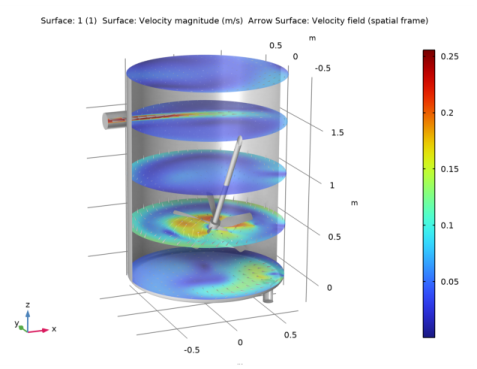
Figure 2 shows the computed velocity field. The inlet stream is seen to propagate through the tank and turn at the opposite wall. Fluid is drawn downward in the vicinity of the impeller. Along the outer walls the fluid in general flows upwards. This implies that a fluid parcel that does not pass close to the outlet when arriving at the bottom will be transported up again along the tank walls.
Figure 2: The frozen rotor flow field in the mixer visualized at five positions.
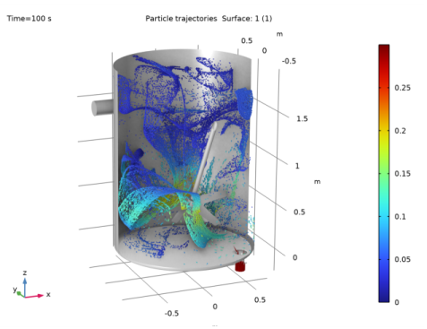
The trajectories of the injected particles after 100 s of simulation time are plotted in Figure 3. Each particle is represented by a cone pointing in direction of the particle velocity. At this time, the particles are distributed throughout the whole vessel, but still mostly in certain bands. Some of the particles are seen to have passed the outlet. These particles are still at the outlet since a freeze condition is applied. The particles are colored by the velocity magnitude. As expected, particles close to the impeller are subjected to higher velocities. However, the highest velocities occur inside the tubular outlet channel.
Figure 3: Flow patterns inside the test apparatus with water at 1 m/s.
By injecting a pulse input of a tracer species into a reactor or mixing vessel, and subsequently measuring the concentration C(t) at the outlet, the residence time distribution function E(t) can be defined as (Ref. 1)
(1)
The residence time distribution function can be said to quantify how much time different fractions of the total amount of species being mixed have spent in the vessel. Using an integral form, the fraction of the tracer species leaving the vessel that have spent between times t1 and t2 inside the vessel can be defined as
(2)
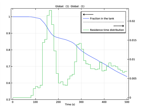
In the present model, the tracer species are as discrete particles, meaning that the concentration at the outlet is not known in each time step. To estimate the concentration, the number of particles that exit the tank over a short time is computed. In Figure 4, the residence time distribution, using a sampling time of 10 s, is plotted. No particles exit before 80 s. There are two notable peaks, at 150 s and 300 s, with significant ejection of particles, before the distribution levels out. The fraction remaining in the tank is also plotted. More than 60% of the particles remain in the tank after 500 s, corresponding to 125 rotations of the impeller.
Figure 4: Residence time distribution for the particles injected into the mixer.
Reference
1. H.S. Fogler, Elements of Chemical Reaction Engineering, 2nd Ed., Prentice-Hall, 1992
Application Library path: Chemical_Reaction_Engineering_Module/Mixing_and_Separation/continuous_mixer
Modeling Instructions
From the File menu, choose New.
New
In the New window, click  Model Wizard.
Model Wizard
1
In the Model Wizard window, click  3D.
2
In the Select Physics tree, select Fluid Flow>Single-Phase Flow>Rotating Machinery, Fluid Flow>Turbulent Flow>Turbulent Flow, k-ε.
3
Click Add.
4
Click  Study.
5
In the Select Study tree, select Preset Studies for Selected Physics Interfaces>Frozen Rotor.
6
Load the model geometry from a geometry sequence.
Geometry 1
1
In the Geometry toolbar, click Insert Sequence and choose Insert Sequence.
2
3
In the Geometry toolbar, click  Build All.
Global Definitions
Parameters 1
1
In the Model Builder window, under Global Definitions click Parameters 1.
2
In the Settings window for Parameters, locate the Parameters section.
3
Click  Load from File.
4
Parameters 2
1
In the Home toolbar, click  Parameters and choose Add>Parameters.
2
In the Settings window for Parameters, locate the Parameters section.
3
Click  Load from File.
4
Definitions
Impeller Blades
1
In the Model Builder window, expand the Component 1 (comp1)>Definitions node.
2
Right-click Definitions and choose Selections>Explicit.
3
In the Settings window for Explicit, type Impeller Blades in the Label text field.
4
Locate the Input Entities section. From the Geometric entity level list, choose Boundary.
5
Blade edges
1
In the Definitions toolbar, click  Explicit.
2
In the Settings window for Explicit, locate the Input Entities section.
3
From the Geometric entity level list, choose Edge.
4
5
In the Label text field, type Blade edges.
Add Material
1
In the Home toolbar, click  Add Material to open the Add Material window.
2
Go to the Add Material window.
3
In the tree, select Built-in>Water, liquid.
4
Click Add to Component in the window toolbar.
5
In the Home toolbar, click  Add Material to close the Add Material window.
Turbulent Flow, k-ε (spf)
1
In the Model Builder window, under Component 1 (comp1) click Turbulent Flow, k-ε (spf).
2
In the Settings window for Turbulent Flow, k-ε, locate the Physical Model section.
3
Select the Include gravity check box.
4
Select the Use reduced pressure check box.
Interior Wall 1
1
In the Model Builder window, expand the Turbulent Flow, k-ε (spf) node.
2
Right-click Component 1 (comp1)>Turbulent Flow, k-ε (spf) and choose Interior Wall.
3
In the Settings window for Interior Wall, locate the Boundary Selection section.
4
From the Selection list, choose Impeller Blades.
Inlet 1
1
In the Physics toolbar, click  Boundaries and choose Inlet.
2
3
In the Settings window for Inlet, locate the Boundary Condition section.
4
From the list, choose Fully developed flow.
5
Clear the Apply condition on each disjoint selection separately check box.
6
Locate the Fully Developed Flow section. In the Uav text field, type v_in.
Outlet 1
1
In the Physics toolbar, click  Boundaries and choose Outlet.
2
Wall 2
1
In the Physics toolbar, click  Boundaries and choose Wall.
2
3
In the Settings window for Wall, locate the Boundary Condition section.
4
From the Wall condition list, choose Slip.
Moving Mesh
In the Model Builder window, expand the Moving Mesh node.
Rotating Domain 1
1
In the Model Builder window, expand the Component 1 (comp1)>Moving Mesh>Rotating Domain 1 node, then click Rotating Domain 1.
2
In the Settings window for Rotating Domain, locate the Domain Selection section.
3
From the Selection list, choose Manual.
4
Click  Clear Selection.
5
6
Locate the Rotation section. From the Rotational velocity expression list, choose Constant angular velocity.
7
In the ω text field, type Omega.
8
Locate the Axis section. Specify the rax vector as
9
Specify the urot vector as
Add Physics
1
In the Physics toolbar, click  Add Physics to open the Add Physics window.
2
Go to the Add Physics window.
3
In the tree, select Fluid Flow>Particle Tracing>Particle Tracing for Fluid Flow (fpt).
4
Click Add to Component 1 in the window toolbar.
5
In the tree, select Fluid Flow>Particle Tracing>Particle Tracing for Fluid Flow (fpt).
6
In the Physics toolbar, click  Add Physics to close the Add Physics window.
Particle Tracing for Fluid Flow (fpt)
1
In the Settings window for Particle Tracing for Fluid Flow, locate the Particle Release and Propagation section.
2
From the Formulation list, choose Massless.
3
Locate the Additional Variables section. Select the Store particle release statistics check box.
Wall 1
1
In the Model Builder window, under Component 1 (comp1)>Particle Tracing for Fluid Flow (fpt) click Wall 1.
2
In the Settings window for Wall, locate the Wall Condition section.
3
From the Wall condition list, choose Disappear.
Particle Properties 1
1
In the Model Builder window, click Particle Properties 1.
2
In the Settings window for Particle Properties, locate the Particle Properties section.
3
Specify the v vector as
Inlet 1
1
In the Physics toolbar, click  Boundaries and choose Inlet.
2
3
In the Settings window for Inlet, locate the Initial Position section.
4
From the Initial position list, choose Random.
5
In the N text field, type nPart.
Outlet 1
1
In the Physics toolbar, click  Boundaries and choose Outlet.
2
Particle Counter 1
1
In the Physics toolbar, click  Boundaries and choose Particle Counter.
2
Mesh 1
Size 1
In the Model Builder window, under Component 1 (comp1) right-click Mesh 1 and choose Size.
Size
1
In the Settings window for Size, locate the Element Size section.
2
From the Predefined list, choose Coarse.
3
Click the Custom button.
4
Locate the Element Size Parameters section. In the Maximum element size text field, type h_dom_max.
5
In the Minimum element size text field, type h_dom_min.
6
In the Maximum element growth rate text field, type h_dom_growth.
7
In the Curvature factor text field, type h_dom_curvef.
8
In the Resolution of narrow regions text field, type h_dom_narrowres.
Size 1
1
In the Model Builder window, click Size 1.
2
In the Settings window for Size, locate the Geometric Entity Selection section.
3
From the Geometric entity level list, choose Boundary.
4
Click to select the  Activate Selection toggle button.
5
6
Locate the Element Size section. From the Predefined list, choose Fine.
7
From the Calibrate for list, choose Fluid dynamics.
8
Click the Custom button.
9
Locate the Element Size Parameters section.
10
Select the Maximum element size check box. In the associated text field, type h_bnd_max.
11
Select the Minimum element size check box. In the associated text field, type h_bnd_min.
12
Select the Curvature factor check box. In the associated text field, type h_bnd_curvef.
Size 2
1
In the Model Builder window, right-click Mesh 1 and choose Size.
2
In the Settings window for Size, locate the Geometric Entity Selection section.
3
From the Geometric entity level list, choose Boundary.
4
From the Selection list, choose Impeller Blades.
5
Locate the Element Size section. From the Predefined list, choose Extra fine.
6
Click the Custom button.
7
Locate the Element Size Parameters section.
8
Select the Maximum element size check box. In the associated text field, type h_bnd_max/2.5.
Free Triangular 1
1
In the Mesh toolbar, click  Boundary and choose Free Triangular.
2
Size 1
1
Right-click Free Triangular 1 and choose Size.
2
In the Settings window for Size, locate the Element Size section.
3
Click the Custom button.
4
Locate the Element Size Parameters section.
5
Select the Maximum element growth rate check box. In the associated text field, type h_inout_growth.
Free Triangular 1
Right-click Free Triangular 1 and choose Size.
Size 2
1
In the Settings window for Size, locate the Geometric Entity Selection section.
2
From the Geometric entity level list, choose Edge.
3
Locate the Element Size section. From the Calibrate for list, choose Fluid dynamics.
4
From the Predefined list, choose Extra fine.
5
6
Click the Custom button.
7
Locate the Element Size Parameters section.
8
Select the Maximum element size check box. In the associated text field, type h_bnd_max*0.45.
Swept 1
1
In the Mesh toolbar, click  Swept.
2
In the Settings window for Swept, locate the Domain Selection section.
3
From the Geometric entity level list, choose Domain.
4
Distribution 1
1
Right-click Swept 1 and choose Distribution.
2
In the Settings window for Distribution, locate the Distribution section.
3
From the Distribution type list, choose Predefined.
4
In the Number of elements text field, type n_inlet.
5
In the Element ratio text field, type n_inlet_hratio.
6
Select the Reverse direction check box.
Swept 2
1
In the Mesh toolbar, click  Swept.
2
In the Settings window for Swept, locate the Domain Selection section.
3
From the Geometric entity level list, choose Domain.
4
Distribution 1
1
Right-click Swept 2 and choose Distribution.
2
In the Settings window for Distribution, locate the Distribution section.
3
From the Distribution type list, choose Predefined.
4
In the Number of elements text field, type n_inlet*2.
5
In the Element ratio text field, type n_inlet_hratio.
Free Triangular 2
1
In the Mesh toolbar, click  Boundary and choose Free Triangular.
2
In the Settings window for Free Triangular, locate the Boundary Selection section.
3
From the Selection list, choose Impeller Blades.
Size 1
1
Right-click Free Triangular 2 and choose Size.
2
In the Settings window for Size, locate the Geometric Entity Selection section.
3
From the Geometric entity level list, choose Edge.
4
From the Selection list, choose Blade edges.
5
Locate the Element Size section. Click the Custom button.
6
Locate the Element Size Parameters section.
7
Select the Maximum element size check box. In the associated text field, type h_blade_max.
8
Select the Minimum element size check box. In the associated text field, type h_blade_min.
Corner Refinement 1
1
In the Mesh toolbar, click  More Attributes and choose Corner Refinement.
2
In the Settings window for Corner Refinement, locate the Domain Selection section.
3
From the Geometric entity level list, choose Domain.
4
Click in the Graphics window and then press Ctrl+A to select all domains.
5
Locate the Boundary Selection section. Click to select the  Activate Selection toggle button.
6
Free Tetrahedral 1
In the Mesh toolbar, click  Free Tetrahedral.
Size 1
1
Right-click Free Tetrahedral 1 and choose Size.
2
In the Settings window for Size, locate the Geometric Entity Selection section.
3
From the Geometric entity level list, choose Domain.
4
5
Locate the Element Size section. Click the Custom button.
6
Locate the Element Size Parameters section.
7
Select the Maximum element growth rate check box. In the associated text field, type h_blade_growth.
Boundary Layers 1
1
In the Mesh toolbar, click  Boundary Layers.
2
In the Settings window for Boundary Layers, locate the Geometric Entity Selection section.
3
From the Geometric entity level list, choose Domain.
4
Click in the Graphics window and then press Ctrl+A to select all domains.
5
Click to expand the Corner Settings section. From the Handling of sharp edges list, choose Trimming.
Boundary Layer Properties
1
In the Model Builder window, click Boundary Layer Properties.
2
In the Settings window for Boundary Layer Properties, locate the Layers section.
3
In the Number of layers text field, type 5.
4
In the Thickness adjustment factor text field, type bl_thicknessf.
5
6
Click  Build All.
Study 1
1
In the Model Builder window, click Study 1.
2
In the Settings window for Study, locate the Study Settings section.
3
Clear the Generate default plots check box.
4
In the Home toolbar, click  Compute.
Add Study
1
In the Home toolbar, click  Add Study to open the Add Study window.
2
Go to the Add Study window.
3
Find the Studies subsection. In the Select Study tree, select General Studies>Time Dependent.
4
Click Add Study in the window toolbar.
5
In the Home toolbar, click  Add Study to close the Add Study window.
Study 2
Step 1: Time Dependent
1
In the Settings window for Time Dependent, locate the Study Settings section.
2
In the Output times text field, type range(0,1,100) range(100+deltaT,deltaT,tEnd).
3
Locate the Physics and Variables Selection section. Select the Modify model configuration for study step check box.
4
In the tree, select Component 1 (comp1)>Turbulent Flow, k-ε (spf).
5
Click  Disable in Solvers.
6
In the tree, select Component 1 (comp1)>Moving Mesh, Controls spatial frame>Rotating Domain 1.
7
Click  Disable.
8
Click  Disable.
9
Click to expand the Values of Dependent Variables section. Find the Values of variables not solved for subsection. From the Settings list, choose User controlled.
10
From the Method list, choose Solution.
11
From the Study list, choose Study 1, Frozen Rotor.
12
In the Home toolbar, click  Compute.
Definitions
Hide for Geometry 1
1
In the Model Builder window, expand the Definitions node.
2
Right-click View 1 and choose Hide for Geometry.
3
In the Settings window for Hide for Geometry, locate the Selection section.
4
From the Geometric entity level list, choose Boundary.
5
On the object igf1, select Boundaries 2, 3, 6, 10, 12, 13, 16–21, 24, 36, 39, 41, 49, and 53 only.
Results
In the Model Builder window, expand the Results node.
Cut Plane 1
1
In the Model Builder window, expand the Results>Datasets node.
2
Right-click Results>Datasets and choose Cut Plane.
3
In the Settings window for Cut Plane, locate the Plane Data section.
4
Select the Additional parallel planes check box.
5
From the Plane list, choose xy-planes.
6
In the Distances text field, type 0.5 1.0 1.5 1.95.
All Walls
1
In the Results toolbar, click  More Datasets and choose Surface.
2
In the Settings window for Surface, type All Walls in the Label text field.
3
Exterior Walls
1
In the Results toolbar, click  More Datasets and choose Surface.
2
In the Settings window for Surface, type Exterior Walls in the Label text field.
3
Interior Walls
1
In the Results toolbar, click  More Datasets and choose Surface.
2
In the Settings window for Surface, type Interior Walls in the Label text field.
3
Velocity (spf)
1
In the Results toolbar, click  3D Plot Group.
2
In the Settings window for 3D Plot Group, type Velocity (spf) in the Label text field.
3
Locate the Plot Settings section. Clear the Plot dataset edges check box.
Surface 1
1
Right-click Velocity (spf) and choose Surface.
2
In the Settings window for Surface, locate the Expression section.
3
In the Expression text field, type 1.
4
Locate the Coloring and Style section. From the Coloring list, choose Uniform.
5
From the Color list, choose Gray.
Surface 2
1
In the Model Builder window, right-click Velocity (spf) and choose Surface.
2
In the Settings window for Surface, locate the Data section.
3
From the Dataset list, choose Cut Plane 1.
Transparency 1
1
In the Model Builder window, right-click Surface 2 and choose Transparency.
2
In the Settings window for Transparency, locate the Transparency section.
3
Set the Transparency value to 0.4.
4
In the Velocity (spf) toolbar, click  Plot.
5
In the Graphics window toolbar, clicknext to  Scene Light, then choose Ambient Occlusion.
Arrow Surface 1
1
In the Model Builder window, right-click Velocity (spf) and choose Arrow Surface.
2
In the Settings window for Arrow Surface, locate the Data section.
3
From the Dataset list, choose Cut Plane 1.
4
Locate the Arrow Positioning section. In the Number of arrows text field, type 900.
5
Locate the Coloring and Style section. From the Arrow type list, choose Cone.
6
From the Color list, choose Gray.
Pressure (spf)
1
In the Home toolbar, click  Add Plot Group and choose 3D Plot Group.
2
In the Settings window for 3D Plot Group, type Pressure (spf) in the Label text field.
3
Locate the Plot Settings section. Clear the Plot dataset edges check box.
Surface 1
1
Right-click Pressure (spf) and choose Surface.
2
In the Settings window for Surface, locate the Data section.
3
From the Dataset list, choose All Walls.
4
Locate the Expression section. In the Expression text field, type 1.
5
Locate the Coloring and Style section. From the Coloring list, choose Uniform.
6
From the Color list, choose Gray.
Pressure
1
In the Model Builder window, right-click Pressure (spf) and choose Contour.
2
In the Settings window for Contour, locate the Data section.
3
From the Dataset list, choose Exterior Walls.
4
Locate the Expression section. In the Expression text field, type p.
5
Locate the Levels section. Clear the Round the levels check box.
6
In the Label text field, type Pressure.
7
Locate the Levels section. In the Total levels text field, type 40.
Upside Pressure
1
Right-click Pressure (spf) and choose Contour.
2
In the Settings window for Contour, type Upside Pressure in the Label text field.
3
Locate the Data section. From the Dataset list, choose Interior Walls.
4
Locate the Levels section. Clear the Round the levels check box.
5
Locate the Expression section. In the Expression text field, type up(p).
6
Locate the Levels section. In the Total levels text field, type 40.
Deformation 1
1
Right-click Upside Pressure and choose Deformation.
2
In the Settings window for Deformation, locate the Expression section.
3
In the x-component text field, type nx/sqrt(up(tremetric)).
4
In the y-component text field, type ny/sqrt(up(tremetric)).
5
In the z-component text field, type nz/sqrt(up(tremetric)).
6
Locate the Scale section.
7
Select the Scale factor check box. In the associated text field, type 0.1.
Downside Pressure
1
In the Model Builder window, right-click Pressure (spf) and choose Contour.
2
In the Settings window for Contour, type Downside Pressure in the Label text field.
3
Locate the Data section. From the Dataset list, choose Interior Walls.
4
Locate the Expression section. In the Expression text field, type down(p).
5
Locate the Levels section. In the Total levels text field, type 40.
6
Clear the Round the levels check box.
Deformation 1
1
Right-click Downside Pressure and choose Deformation.
2
In the Settings window for Deformation, locate the Expression section.
3
In the x-component text field, type -nx/sqrt(down(tremetric)).
4
In the y-component text field, type -ny/sqrt(down(tremetric)).
5
In the z-component text field, type -nz/sqrt(down(tremetric)).
6
Locate the Scale section.
7
Select the Scale factor check box. In the associated text field, type 0.1.
Wall Resolution (spf)
1
In the Home toolbar, click  Add Plot Group and choose 3D Plot Group.
2
In the Settings window for 3D Plot Group, type Wall Resolution (spf) in the Label text field.
Wall Resolution
1
Right-click Wall Resolution (spf) and choose Surface.
2
In the Settings window for Surface, type Wall Resolution in the Label text field.
3
Locate the Data section. From the Dataset list, choose Exterior Walls.
4
Locate the Expression section. In the Expression text field, type spf.Delta_wPlus.
Wall Resolution (spf)
In the Model Builder window, click Wall Resolution (spf).
Wall Resolution, Interior Walls
1
In the Wall Resolution (spf) toolbar, click  More Plots and choose Surface Slit.
2
In the Settings window for Surface Slit, type Wall Resolution, Interior Walls in the Label text field.
3
In the Model Builder window, click Wall Resolution, Interior Walls.
4
In the Label text field, type Wall Resolution, Interior Walls.
5
Locate the Data section. From the Dataset list, choose Interior Walls.
6
Locate the Expression on the Upside section. In the Expression text field, type spf.Delta_wPlus_u.
7
Locate the Expression on the Downside section. In the Expression text field, type spf.Delta_wPlus_d.
Residence time distribution
1
In the Home toolbar, click  Add Plot Group and choose 1D Plot Group.
2
In the Settings window for 1D Plot Group, type Residence time distribution in the Label text field.
3
Locate the Data section. From the Dataset list, choose Study 2/Solution 2 (sol2).
4
From the Time selection list, choose Interpolated.
5
In the Times (s) text field, type range(0,deltaT,tEnd).
Global 1
1
Right-click Residence time distribution and choose Global.
2
In the Settings window for Global, locate the y-Axis Data section.
3
Global 2
1
In the Model Builder window, right-click Residence time distribution and choose Global.
2
In the Settings window for Global, locate the y-Axis Data section.
3
4
In the Residence time distribution toolbar, click  Plot.
Residence time distribution
1
In the Model Builder window, click Residence time distribution.
2
In the Settings window for 1D Plot Group, locate the Plot Settings section.
3
Select the Two y-axes check box.
4
In the table, select the Plot on secondary y-axis check box for Global 2.
5
Locate the Axis section. Select the Manual axis limits check box.
6
In the y minimum text field, type 0.5.
7
In the y maximum text field, type 1.05.
8
Locate the Grid section. Select the Manual spacing check box.
9
In the x spacing text field, type 100.
10
In the y spacing text field, type 0.1.
11
In the Secondary y spacing text field, type 0.005.
Global 1
1
In the Model Builder window, click Global 1.
2
In the Settings window for Global, click to expand the Legends section.
3
From the Legends list, choose Manual.
4
Global 2
1
In the Model Builder window, click Global 2.
2
In the Settings window for Global, click to expand the Coloring and Style section.
3
From the Function type list, choose Discrete.
4
Click to expand the Legends section. From the Legends list, choose Manual.
5
6
Click to collapse the Legends section. In the Residence time distribution toolbar, click  Plot.
Particle Trajectories (fpt)
1
In the Model Builder window, under Results click Particle Trajectories (fpt).
2
In the Settings window for 3D Plot Group, locate the Data section.
3
From the Time (s) list, choose 100.
4
Locate the Plot Settings section. Clear the Plot dataset edges check box.
Surface 1
Right-click Particle Trajectories (fpt) and choose Surface.
Surface 1
1
In the Model Builder window, expand the Results>Particle Trajectories (fpt) node, then click Surface 1.
2
In the Settings window for Surface, locate the Expression section.
3
In the Expression text field, type 1.
4
Locate the Coloring and Style section. From the Coloring list, choose Uniform.
5
From the Color list, choose Gray.
Particle Trajectories 1
1
In the Model Builder window, click Particle Trajectories 1.
2
In the Settings window for Particle Trajectories, locate the Coloring and Style section.
3
Find the Point style subsection. From the Type list, choose Comet tail.
Color Expression 1
1
In the Model Builder window, expand the Particle Trajectories 1 node, then click Color Expression 1.
2
In the Settings window for Color Expression, click to expand the Range section.
3
Select the Manual color range check box.
4
In the Maximum text field, type 0.3.
5
In the Minimum text field, type 0.
6
In the Particle Trajectories (fpt) toolbar, click  Plot.
Geometry Modeling Instructions
Follow steps below to generate the geometry used in this model.
Add Component
In the Home toolbar, click  Add Component and choose 3D.
Global Definitions
Parameters 1
1
In the Model Builder window, under Global Definitions click Parameters 1.
2
In the Settings window for Parameters, locate the Parameters section.
3
Part Libraries
1
In the Home toolbar, click  Windows and choose Part Libraries.
2
In the Model Builder window, under Component 1 (comp1) click Geometry 1.
3
In the Part Libraries window, select Mixer Module>Tanks>flat_bottom_tank in the tree.
4
Click  Add to Geometry.
Geometry 1
Flat Bottom Tank 1 (pi1)
1
In the Model Builder window, under Component 1 (comp1)>Geometry 1 click Flat Bottom Tank 1 (pi1).
2
In the Settings window for Part Instance, locate the Input Parameters section.
3
Union 1 (uni1)
1
In the Geometry toolbar, click  Booleans and Partitions and choose Union.
2
3
In the Settings window for Union, locate the Union section.
4
Clear the Keep interior boundaries check box.
5
Click  Build Selected.
Part Libraries
1
In the Geometry toolbar, click  Parts and choose Part Libraries.
2
In the Model Builder window, click Geometry 1.
3
In the Part Libraries window, select Mixer Module>Shafts>impeller_shaft in the tree.
4
Click  Add to Geometry.
Geometry 1
Impeller Shaft 1 (pi2)
1
In the Model Builder window, under Component 1 (comp1)>Geometry 1 click Impeller Shaft 1 (pi2).
2
In the Settings window for Part Instance, locate the Input Parameters section.
3
Part Libraries
1
In the Geometry toolbar, click  Parts and choose Part Libraries.
2
In the Model Builder window, click Geometry 1.
3
In the Part Libraries window, select Mixer Module>Impellers, Axial>pitched_blade_impeller_constant_pitch in the tree.
4
Click  Add to Geometry.
Geometry 1
Pitched Blade Impeller with Constant Pitch 1 (pi3)
1
In the Model Builder window, under Component 1 (comp1)>Geometry 1 click Pitched Blade Impeller with Constant Pitch 1 (pi3).
2
In the Settings window for Part Instance, locate the Input Parameters section.
3
Rotate 1 (rot1)
1
In the Geometry toolbar, click  Transforms and choose Rotate.
2
Select the objects pi2, pi3(1), and pi3(2) only.
3
In the Settings window for Rotate, locate the Rotation section.
4
From the Axis type list, choose x-axis.
5
In the Angle text field, type impellerTilt.
6
Locate the Point on Axis of Rotation section. In the z text field, type 0.5.
7
Click  Build Selected.
Move 1 (mov1)
1
In the Geometry toolbar, click  Transforms and choose Move.
2
Select the objects rot1(1), rot1(2), and rot1(3) only.
3
In the Settings window for Move, locate the Displacement section.
4
In the y text field, type -0.175.
Difference 1 (dif1)
1
In the Geometry toolbar, click  Booleans and Partitions and choose Difference.
2
Select the objects mov1(3) and uni1 only.
3
In the Settings window for Difference, locate the Difference section.
4
Find the Objects to subtract subsection. Click to select the  Activate Selection toggle button.
5
Select the objects mov1(1) and mov1(2) only.
Cylinder 1 (cyl1)
1
In the Geometry toolbar, click  Cylinder.
2
In the Settings window for Cylinder, locate the Size and Shape section.
3
In the Radius text field, type r_in.
4
In the Height text field, type r_in*8.
5
Locate the Position section. In the x text field, type -0.9.
6
In the y text field, type 0.3.
7
In the z text field, type 1.5.
8
Locate the Axis section. From the Axis type list, choose x-axis.
Work Plane 1 (wp1)
1
In the Geometry toolbar, click  Work Plane.
2
In the Settings window for Work Plane, locate the Plane Definition section.
3
From the Plane list, choose xz-plane.
4
In the y-coordinate text field, type -0.35.
Work Plane 1 (wp1)>Plane Geometry
In the Model Builder window, click Plane Geometry.
Work Plane 1 (wp1)>Rectangle 1 (r1)
1
In the Work Plane toolbar, click  Rectangle.
2
In the Settings window for Rectangle, locate the Size and Shape section.
3
In the Width text field, type 0.2.
4
In the Height text field, type 0.2.
5
Locate the Position section. In the xw text field, type 0.25.
6
In the yw text field, type -0.25.
Work Plane 1 (wp1)>Rectangle 2 (r2)
1
In the Work Plane toolbar, click  Rectangle.
2
In the Settings window for Rectangle, locate the Size and Shape section.
3
In the Width text field, type 0.25.
4
In the Height text field, type 0.2.
5
Locate the Position section. In the xw text field, type 0.25.
6
In the yw text field, type -0.25.
Work Plane 1 (wp1)>Fillet 1 (fil1)
1
In the Work Plane toolbar, click  Fillet.
2
On the object r1, select Point 3 only.
3
In the Settings window for Fillet, locate the Radius section.
4
In the Radius text field, type 0.03.
Work Plane 1 (wp1)>Difference 1 (dif1)
1
In the Work Plane toolbar, click  Booleans and Partitions and choose Difference.
2
3
In the Settings window for Difference, locate the Difference section.
4
Find the Objects to subtract subsection. Click to select the  Activate Selection toggle button.
5
Geometry 1
Work Plane 1 (wp1)
In the Model Builder window, collapse the Component 1 (comp1)>Geometry 1>Work Plane 1 (wp1) node.
Revolve 1 (rev1)
1
In the Model Builder window, right-click Geometry 1 and choose Revolve.
2
In the Settings window for Revolve, locate the Revolution Axis section.
3
Find the Point on the revolution axis subsection. In the xw text field, type 0.5.
4
In the yw text field, type -0.25.
5
Locate the Revolution Angles section. Clear the Keep original faces check box.
6
In the Geometry toolbar, click  Build All.
Ignore Edges 1 (ige1)
1
In the Geometry toolbar, click  Virtual Operations and choose Ignore Edges.
2
In the Settings window for Ignore Edges, locate the Input section.
3
Click  Paste Selection.
4
In the Paste Selection dialog box, type 13, 27-29, 60, 85, 88, 90, 96, 97, 99, 101, 105, 109, 115, 116, 120, 121, 147, 148, 171, 180, 188, 189, 197, 198 in the Selection text field.
5
Ignore Faces 1 (igf1)
1
In the Geometry toolbar, click  Virtual Operations and choose Ignore Faces.
2
In the Settings window for Ignore Faces, locate the Input section.
3
Click  Paste Selection.
4
In the Paste Selection dialog box, type 51 in the Selection text field.
5
6
In the Geometry toolbar, click  Build All.