PDF

Water Purification Reactor
Introduction
Water purification for turning natural water into drinking water is a process constituted of several steps. At least one step must be a disinfectant step. One way to achieve efficient disinfection in an environmentally friendly way is to use ozone. A typical ozone purification reactor is about 40 m long and resembles a maze with partial walls or baffles that divide the space into room-sized compartments (Ref. 1). When water flows through the reactor turbulent flow is created along its winding path around the baffles toward the exit pipe. The turbulence mixes the water with ozone gas that enters through diffusers just long enough to deactivate micropollutants. When the water leaves the reactor, the remaining purification steps filter off or otherwise remove the reacted pollutants.
When analyzing an ozone purification reactor, the first step is to get an overview of the turbulent flow field. The results from the turbulent-flow simulation can then be used for further analyses of residence time and chemical species transport and reactions by adding more physics to the model. The current model solves for turbulent flow in a water treatment reactor using the Turbulent Flow, k-ε interface.
Model Definition
Model Geometry
The model geometry along with some boundary conditions are shown in Figure 1. The full reactor has a symmetry plane which is utilized to reduce the size of the model.
Figure 1: Model geometry. All boundaries except the inlet, outlet, and symmetry plane are walls.
Domain Equations and Boundary Conditions
Based on the inlet velocity and diameter, which in this case correspond to 0.1 m/s and 0.4 m respectively, the Reynolds number is
Here ν is the kinematic viscosity. The high Reynolds number clearly indicates that the flow is turbulent. This means that the flow must be modeled using a turbulence model. In this case, the k-ε turbulence model is used, as it is often done in industrial applications, much because it is both relatively robust and computationally inexpensive compared to more advanced turbulence models. One major reason to why the k-ε model is inexpensive is that it makes use of wall functions to describe the flow close to walls instead of resolving the very steep gradients there. All boundaries in Figure 1, except the inlet, the outlet, and the symmetry plane, are walls.
The fully developed flow is used as inlet boundary condition. A constant pressure is prescribed on the outlet.
Notes About the COMSOL Implementation
Three-dimensional turbulent flows can take a rather long time to solve, even when using a turbulence models with wall functions. To make this tutorial feasible, the mesh is deliberately selected to be relatively coarse and the results are therefore not mesh independent. In any model, the effect or refining the mesh should be investigated in order to ensure that the model is well resolved.
Results and Discussion
Figure 2 shows the velocity field in the symmetry plane. The jet from the inlet hits the top of the first baffle which splits the jet. One half creates a strong recirculation zone in the first “chamber”. The other half continues down into the reactor and gradually spreads out. The velocity magnitude decreases as more fluid is entrained into the jet.
Figure 2: Velocity field in the symmetry plane.
Figure 3 gives a more complete picture of the mixing process in the reactor. The streamlines are colored by the velocity magnitude, and their width are proportional to the turbulent viscosity. Wide lines hence indicate high degree of mixing. The turbulence in this example is mainly produced in the shear layers between the central jet and the recirculation zones. The mixing can be seen to be relatively weak in the beginning of the reactor. The plot also shows that it increases further downstream.
Figure 3: Streamlines colored by velocity. The width of the streamlines are proportional to the turbulent viscosity.
Reference
1. J. Hofman, D. Wind, B. Wols, W. Uijttewaal, H. van Dijk, and G. Stelling, “The use of CFD Modeling to determine the influence of residence time distribution on the disinfection of drinking water in ozone contactors,” COMSOL Conference 2007, Grenoble, 2007; https://www.comsol.com/stories/hofman_water_purification/full/
Application Library path: CFD_Module/Single-Phase_Flow/water_purification_reactor
Modeling Instructions
From the File menu, choose New.
New
In the New window, click  Model Wizard.
Model Wizard
1
In the Model Wizard window, click  3D.
2
In the Select Physics tree, select Fluid Flow>Single-Phase Flow>Turbulent Flow>Turbulent Flow, k-ε (spf).
3
Click Add.
4
Click  Study.
5
In the Select Study tree, select General Studies>Stationary.
6
Global Definitions
Parameters 1
1
In the Model Builder window, under Global Definitions click Parameters 1.
2
In the Settings window for Parameters, locate the Parameters section.
3
Geometry 1
You can build the reactor geometry from geometric primitives. Here, instead, use a file containing the sequence of geometry features that has been provided for convenience.
1
In the Geometry toolbar, click Insert Sequence and choose Insert Sequence.
2
3
In the Geometry toolbar, click  Build All.
The model geometry is now complete (Figure 1).
Add Material
1
In the Home toolbar, click  Add Material to open the Add Material window.
2
Go to the Add Material window.
3
In the tree, select Built-in>Water, liquid.
4
Click Add to Component in the window toolbar.
5
In the Home toolbar, click  Add Material to close the Add Material window.
Turbulent Flow, k-ε (spf)
Inlet 1
1
In the Model Builder window, under Component 1 (comp1) right-click Turbulent Flow, k-ε (spf) and choose Inlet.
2
3
In the Settings window for Inlet, locate the Boundary Condition section.
4
From the list, choose Fully developed flow.
5
Locate the Fully Developed Flow section. In the Uav text field, type u_in.
Symmetry 1
1
In the Physics toolbar, click  Boundaries and choose Symmetry.
2
Outlet 1
1
In the Physics toolbar, click  Boundaries and choose Outlet.
2
Mesh 1
1
In the Model Builder window, under Component 1 (comp1) click Mesh 1.
2
In the Settings window for Mesh, locate the Physics-Controlled Mesh section.
3
From the Element size list, choose Coarser.
Size
Right-click Component 1 (comp1)>Mesh 1 and choose Edit Physics-Induced Sequence.
Size 1
In the Model Builder window, right-click Size 1 and choose Disable.
Boundary Layer Properties 1
1
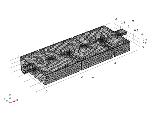
In the Model Builder window, expand the Component 1 (comp1)>Mesh 1>Boundary Layers 1 node, then click Boundary Layer Properties 1.
2
In the Settings window for Boundary Layer Properties, locate the Layers section.
3
In the Number of layers text field, type 2.
4
In the Thickness adjustment factor text field, type 6.
5
In the Model Builder window, collapse the Mesh 1 node.
6
In the Settings window for Mesh, click  Build All.
7
Click the  Zoom Extents button in the Graphics toolbar.
Confirm that the mesh matches the figure below.
Next, solve for the flow field. This takes approximately 15 minutes on a quad-core desktop computer.
Study 1
In the Home toolbar, click  Compute.
Results
The following steps reproduce Figure 2.
First, create a dataset that corresponds to the inlet, outlet, and symmetry plane.
Surface 2
1
In the Results toolbar, click  More Datasets and choose Surface.
2
Slice
1
In the Model Builder window, expand the Results>Velocity (spf) node.
2
Right-click Slice and choose Disable.
Velocity (spf)
1
In the Model Builder window, click Velocity (spf).
2
In the Settings window for 3D Plot Group, locate the Data section.
3
From the Dataset list, choose Surface 2.
Surface 1
1
Right-click Velocity (spf) and choose Surface.
2
In the Settings window for Surface, locate the Data section.
3
From the Dataset list, choose Exterior Walls.
4
Locate the Coloring and Style section. From the Coloring list, choose Uniform.
5
From the Color list, choose Gray.
Surface 2
Right-click Velocity (spf) and choose Surface.
Arrow Surface 1
1
Right-click Velocity (spf) and choose Arrow Surface.
2
In the Settings window for Arrow Surface, locate the Coloring and Style section.
3
From the Arrow length list, choose Logarithmic.
4
Select the Scale factor check box. In the associated text field, type 1.4.
5
Locate the Arrow Positioning section. In the Number of arrows text field, type 300.
6
Locate the Coloring and Style section. From the Color list, choose White.
Velocity (spf)
1
In the Model Builder window, click Velocity (spf).
2
In the Settings window for 3D Plot Group, click to expand the Title section.
3
From the Title type list, choose Manual.
4
In the Title text area, type Velocity field.
5
In the Velocity (spf) toolbar, click  Plot.
6
Click the  Zoom Extents button in the Graphics toolbar.
Proceed to reproduce Figure 3 as follows.
Surface 1
In the Model Builder window, right-click Surface 1 and choose Copy.
3D Plot Group 4
In the Home toolbar, click  Add Plot Group and choose 3D Plot Group.
Surface 1
Right-click 3D Plot Group 4 and choose Paste Surface.
Streamline 1
1
In the Model Builder window, right-click 3D Plot Group 4 and choose Streamline.
2
3
In the Settings window for Streamline, locate the Streamline Positioning section.
4
In the Number text field, type 45.
5
Locate the Coloring and Style section. Find the Line style subsection. From the Type list, choose Ribbon.
6
In the Width expression text field, type spf.nuT*1[s/m].
7
Select the Width scale factor check box. In the associated text field, type 100.
Color Expression 1
1
Right-click Streamline 1 and choose Color Expression.
2
In the Settings window for Color Expression, click to expand the Range section.
3
Select the Manual color range check box.
4
In the Minimum text field, type 0.
5
In the Maximum text field, type 0.1.
Streamlines
1
In the Model Builder window, under Results click 3D Plot Group 4.
2
In the Settings window for 3D Plot Group, locate the Title section.
3
From the Title type list, choose Manual.
4
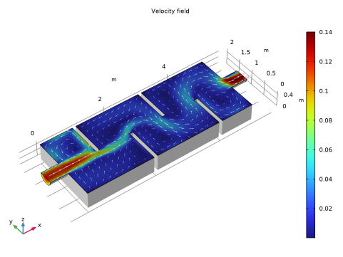
In the Title text area, type Streamlines colored by velocity, width proportional to turbulent viscosity.
5
In the 3D Plot Group 4 toolbar, click  Plot.
6
Click the  Zoom Extents button in the Graphics toolbar.
7
In the Label text field, type Streamlines.