PDF

Bubble-Induced Entrainment Between Stratified Liquid Layers
Introduction
Three-phase flows occur in numerous industrial applications, in free and porous media (nuclear safety, petroleum engineering, and so on). Many biomedical and chemical processes involve mixtures of three or more fluids, for example double emulsions, which play critical roles in applications such as prolonged drug delivery systems, entrapment of vitamins and flavor encapsulation for food additives. Considering a configuration of two immiscible liquids in stratified layers, it is known that a gas bubble of sufficient size rising through the stratified layers can entrain some of the heavier liquid from the lower layer into its wake and transport it to the upper layer of lighter liquid. This entrainment phenomenon has significant effects on both heat and mass transfer, and is encountered in a number of industrial applications. For example, in chemical processing, gas bubbles are sometimes released into pools of stratified liquids to induce mixing and phase transport. In nuclear-reactor safety applications, bubbles of non-condensable gas rise through stratified liquid pools of molten fuel and materials. In metallurgical processing, bubbles of oxygen and other gases may bubble through pools of molten metal with overlying pools of molten silica slag (Ref. 1).
However, computational models for direct simulation of three-phase flow are rather rare in comparison with the large body of research on two-phase flow. The current model, based on the predefined multiphysics coupling between the Laminar flow and Ternary phase field interfaces, simulates three-phase flow (gas and two liquids) with large density and viscosity differences.
This benchmark model simulates a single gas bubble which rises through the interface between two stratified liquid layers thereby inducing entertainment, and validates the results against literature (Ref. 2).
Model Setup
When a gas bubble rises in a two-stratified-liquid-layers configuration, the bubble can either become captured at the interface, or penetrate into the light phase, possibly leading to entrainment of the heavy phase. The criterion is based on a macroscopic balance between buoyancy and surface tension forces, and states that the bubble will penetrate the liquid-liquid interface, if its volume, V, satisfies (Ref. 2),
where g denotes the gravity constant, σ denotes the surface tension, and 1, 2, 3 are the suffixes for gas, heavy liquid, and light liquid, respectively. This criterion has been validated both experimentally and numerically (Ref. 1, Ref. 2).
This model is one of the case considered in Ref. 2. The physical properties of the fluids used in the simulation are listed in Table 1 and Table 2.
(between the two liquids)
Inserting the physical parameters above in Equation  gives Vc = 8.8726·108 kg/m3. Because the volume of a sphere is given by V = 4πr3/3, the critical bubble radius can be estimated to be rc = 2.778 mm.
The radius of the bubble in the simulation is r = mm. Since r > rc, the gas bubble will penetrate the liquid-liquid interface. Due to its relatively large volume, it will furthermore entrain some of the heavy liquid into its wake and transport it into the light liquid forming small droplets of heavy liquid in the upper layer. The mobility M0, which is taken as a function of the phase field variables, is defined in such a way that it becomes zero in each pure phase, , where Mconst = 2·105 m3/s.
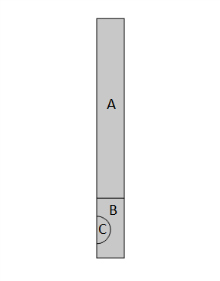
The model is axisymmetric; Figure 1 shows its geometry. The mesh contains around 36150 elements with linear shape functions. The simulation time interval is between 0 and 0.65 s, which is around the time the bubble needs to rise through the given column.
Figure 1: Geometry of the computation domain.
Results and Discussion
The simulation results are shown in Figure 2. Initially, a gas bubble is placed underneath the surface between a heavy liquid and a light liquid, see Figure 2(a). The gas bubble then passes into the upper pool and a volume of heavy liquid is clearly seen to be entrained in its wake, having been pulled through the interfaces between the two liquid layers, see Figure 2(b). If the bubble were of insufficient size, the levitated column would fall back to the lower pool and the gas bubble would continue to rise through the upper pool without having caused any entrainment. This is not the case in current model. Here, the size of the bubble is sufficiently large that the levitated liquid column rises to a height such that it eventually pinches off from the lower layer, see Figure 2(c). As the column elongates, it becomes hydro-dynamically unstable and pinches off into a series of small droplets. A small amount of the heavy liquid adheres to the bubble, see Figure 2(d), and can be considered to have been successfully entrained into the upper fluid layer.
Figure 2: Processing of bubble-induced entrainment between stratified liquid layers. The silver and pink surfaces represent the interfaces between gas and light liquid and between light liquid and heavy liquid, respectively. The colored surface half-enclosing the domain represents the velocity field magnitude.
Figure 3: History of mass changes.
It is important that the mass of each phase is conserved to within a tolerance given by the numerical method and the computational mesh. The mass conservation history is shown in Figure 3. It is observed that the mass loss for the two liquid phases is about 0.1%, and that of the gas phase is about 1.5%. The mass loss of gas is the largest because its volume fraction is much smaller than the other two phases, whereby its relative change becomes most noticeable.
References
1. G.A. Green, J.C. Chen, and M.T. Conlin, “Bubble induced entrainment between stratified liquid layers,” International Journal of Heat and Mass Transfer, vol. 34, pp 149–157, 1991.
2. F. Boyer, C. Lapuerta, S. Minjeaud, B. Piar, and M. Quintard, “Cahn-Hilliard/Navier-Stokes Model for the Simulation of Three-Phase Flows,” Transport in Porous Media, vol. 82, pp 463–483, 2010.
Application Library path: CFD_Module/Verification_Examples/three_phase_bubble
Modeling Instructions
From the File menu, choose New.
New
In the New window, click  Model Wizard.
Model Wizard
1
In the Model Wizard window, click  2D Axisymmetric.
2
In the Select Physics tree, select Fluid Flow>Multiphase Flow>Three-Phase Flow, Phase Field>Laminar Three-Phase Flow, Phase Field.
3
Click Add.
4
Click  Study.
5
In the Select Study tree, select General Studies>Time Dependent.
6
Geometry 1
1
In the Model Builder window, under Component 1 (comp1) click Geometry 1.
2
In the Settings window for Geometry, locate the Units section.
3
From the Length unit list, choose cm.
Global Definitions
Parameters 1
1
In the Model Builder window, under Global Definitions click Parameters 1.
2
In the Settings window for Parameters, locate the Parameters section.
3
Click  Load from File.
4
Definitions
Variables 1
1
In the Model Builder window, under Component 1 (comp1) right-click Definitions and choose Variables.
2
In the Settings window for Variables, locate the Variables section.
3
Click  Load from File.
4
Geometry 1
Rectangle 1 (r1)
1
In the Model Builder window, expand the Component 1 (comp1)>Geometry 1 node.
2
Right-click Geometry 1 and choose Rectangle.
3
In the Settings window for Rectangle, locate the Size and Shape section.
4
In the Width text field, type width/2.
5
In the Height text field, type height.
6
Locate the Position section. From the Base list, choose Center.
7
In the r text field, type width/4.
8
In the z text field, type center_rec.
Circle 1 (c1)
1
In the Geometry toolbar, click  Circle.
2
In the Settings window for Circle, locate the Size and Shape section.
3
In the Radius text field, type radius.
4
In the Sector angle text field, type 180.
5
Locate the Position section. In the z text field, type center_bub.
6
Locate the Rotation Angle section. In the Rotation text field, type -90.
Polygon 1 (pol1)
1
In the Geometry toolbar, click  Polygon.
2
In the Settings window for Polygon, locate the Coordinates section.
3
Form Union (fin)
In the Geometry toolbar, click  Build All.
Ternary Phase Field (terpf)
Mixture Properties 1
1
In the Model Builder window, under Component 1 (comp1)>Ternary Phase Field (terpf) click Mixture Properties 1.
2
In the Settings window for Mixture Properties, locate the Phase Field Parameters section.
3
In the M0 text field, type M0.
4
Locate the Surface Tension section. From the Surface tension coefficient of interface between phase A and phase B list, choose User defined. In the σA,B text field, type sigma_AB.
5
From the Surface tension coefficient of interface between phase B and phase C list, choose User defined. In the σB,C text field, type sigma_BC.
6
From the Surface tension coefficient of interface between phase A and phase C list, choose User defined. In the σA,C text field, type sigma_AC.
Initial Values 2
1
In the Physics toolbar, click  Domains and choose Initial Values.
2
3
In the Settings window for Initial Values, locate the Initial Values section.
4
In the phiB text field, type 1.
Initial Values 3
1
In the Physics toolbar, click  Domains and choose Initial Values.
2
Initial Values 1
1
In the Model Builder window, click Initial Values 1.
2
In the Settings window for Initial Values, locate the Initial Values section.
3
In the phiA text field, type 1.
Multiphysics
Three-Phase Flow, Phase Field 1 (tfpf1)
1
In the Model Builder window, under Component 1 (comp1)>Multiphysics click Three-Phase Flow, Phase Field 1 (tfpf1).
2
In the Settings window for Three-Phase Flow, Phase Field, locate the Material Properties section.
3
Click  Add Multiphase Material.
Materials
Fluid A
1
In the Model Builder window, under Component 1 (comp1)>Materials>Multiphase Material 1 (mpmat1) click Phase 1 (mpmat1.phase1).
2
In the Settings window for Phase, locate the Material Contents section.
3
4
In the Label text field, type Fluid A.
Fluid B
1
In the Model Builder window, under Component 1 (comp1)>Materials>Multiphase Material 1 (mpmat1) click Phase 2 (mpmat1.phase2).
2
In the Settings window for Phase, type Fluid B in the Label text field.
3
Locate the Material Contents section. In the table, enter the following settings:
Fluid C
1
In the Model Builder window, click Phase 3 (mpmat1.phase3).
2
In the Settings window for Phase, locate the Material Contents section.
3
4
In the Label text field, type Fluid C.
Definitions
Ramp 1 (rm1)
1
In the Home toolbar, click  Functions and choose Global>Ramp.
2
In the Settings window for Ramp, locate the Parameters section.
3
In the Slope text field, type 200.
4
Select the Cutoff check box.
5
Laminar Flow (spf)
1
In the Model Builder window, under Component 1 (comp1) click Laminar Flow (spf).
2
In the Settings window for Laminar Flow, locate the Physical Model section.
3
Select the Include gravity check box.
Gravity 1
1
In the Model Builder window, under Component 1 (comp1)>Laminar Flow (spf) click Gravity 1.
2
In the Settings window for Gravity, locate the Acceleration of Gravity section.
3
Specify the g vector as
Pressure Point Constraint 1
1
In the Physics toolbar, click  Points and choose Pressure Point Constraint.
2
Mesh 1
1
In the Model Builder window, under Component 1 (comp1) click Mesh 1.
2
In the Settings window for Mesh, locate the Sequence Type section.
3
From the list, choose User-controlled mesh.
Size
1
In the Model Builder window, under Component 1 (comp1)>Mesh 1 click Size.
2
In the Settings window for Size, locate the Element Size section.
3
Click the Custom button.
4
Locate the Element Size Parameters section. In the Maximum element size text field, type 0.04.
5
Click  Build All.
Study 1
Step 1: Time Dependent
1
In the Model Builder window, under Study 1 click Step 1: Time Dependent.
2
In the Settings window for Time Dependent, locate the Study Settings section.
3
In the Output times text field, type range(0,0.025,1)*0.65.
Solution 1 (sol1)
In the Study toolbar, click  Show Default Solver.
Step 1: Time Dependent
1
In the Model Builder window, under Study 1 click Step 1: Time Dependent.
2
In the Settings window for Time Dependent, click to expand the Results While Solving section.
3
Select the Plot check box.
4
From the Update at list, choose Time steps taken by solver.
5
Click to expand the Values of Dependent Variables section.
Solution 1 (sol1)
1
In the Model Builder window, expand the Study 1>Solver Configurations>Solution 1 (sol1) node, then click Time-Dependent Solver 1.
2
In the Settings window for Time-Dependent Solver, click to expand the Time Stepping section.
3
From the Maximum step constraint list, choose Constant.
4
In the Maximum step text field, type 0.0005.
Results
1
In the Model Builder window, expand the Results node.
2
Right-click Study 1>Solver Configurations>Solution 1 (sol1)>Time-Dependent Solver 1 and choose Get Initial Value.
Study 1
Step 1: Time Dependent
1
In the Settings window for Time Dependent, locate the Results While Solving section.
2
From the Plot group list, choose 2D Plot Group: Three Phases (terpf).
3
In the Study toolbar, click  Compute.
Results
3D Plot Group 8
In the Home toolbar, click  Add Plot Group and choose 3D Plot Group.
Isosurface 1
1
Right-click 3D Plot Group 8 and choose Isosurface.
2
In the Settings window for Isosurface, locate the Expression section.
3
In the Expression text field, type phiB.
4
Locate the Levels section. From the Entry method list, choose Levels.
5
In the Levels text field, type 0.5.
6
Click to expand the Title section. From the Title type list, choose None.
7
Locate the Coloring and Style section. From the Coloring list, choose Uniform.
8
Clear the Color legend check box.
9
From the Color list, choose Magenta.
Isosurface 2
1
In the Model Builder window, right-click 3D Plot Group 8 and choose Isosurface.
2
In the Settings window for Isosurface, locate the Expression section.
3
In the Expression text field, type terpf.phiC.
4
Locate the Levels section. From the Entry method list, choose Levels.
5
In the Levels text field, type 0.5.
6
Locate the Coloring and Style section. From the Coloring list, choose Uniform.
7
Locate the Title section. From the Title type list, choose None.
8
Locate the Coloring and Style section. Clear the Color legend check box.
9
From the Color list, choose Gray.
10
In the 3D Plot Group 8 toolbar, click  Plot.
Slice 1
1
Right-click 3D Plot Group 8 and choose Slice.
2
In the Settings window for Slice, locate the Plane Data section.
3
In the Planes text field, type 1.
4
From the Plane list, choose zx-planes.
5
In the Planes text field, type 1.
Deformation 1
1
Right-click Slice 1 and choose Deformation.
2
In the Settings window for Deformation, locate the Expression section.
3
From the Coordinate system list, choose Global Cartesian.
4
In the x-component text field, type 0.
5
In the y-component text field, type sqrt(0.016^2-r^2).
6
In the z-component text field, type 0.
7
Locate the Scale section.
8
Select the Scale factor check box. In the associated text field, type 1.
9
In the 3D Plot Group 8 toolbar, click  Plot.
3D Plot Group 8
1
In the Model Builder window, under Results click 3D Plot Group 8.
2
In the Settings window for 3D Plot Group, locate the Data section.
3
From the Time (s) list, choose 0.
4
Locate the Color Legend section. Clear the Show legends check box.
5
Click to expand the Title section. From the Title type list, choose None.
6
In the 3D Plot Group 8 toolbar, click  Plot.
7
Locate the Data section. From the Time (s) list, choose 0.21125.
8
In the 3D Plot Group 8 toolbar, click  Plot.
9
From the Time (s) list, choose 0.40625.
10
In the 3D Plot Group 8 toolbar, click  Plot.
11
From the Time (s) list, choose 0.60125.
12
In the 3D Plot Group 8 toolbar, click  Plot.
Surface Integration 1
1
In the Results toolbar, click  More Derived Values and choose Integration>Surface Integration.
Integrate the volume fractions over the whole domain and divide by the initial volume of each phase to see how well the different volumes are conserved during simulation.
2
In the Settings window for Surface Integration, locate the Selection section.
3
From the Selection list, choose All domains.
4
Locate the Expressions section. In the table, enter the following settings:
5
Click  Evaluate.
Table
1
Go to the Table window.
2
Click Table Graph in the window toolbar.
Results
Table Graph 1
1
In the Model Builder window, under Results>1D Plot Group 9 click Table Graph 1.
2
In the Settings window for Table Graph, click to expand the Legends section.
3
Select the Show legends check box.
4
From the Legends list, choose Manual.
5