1D Step Bearing

This benchmark model computes the load-carrying capacity of a one-dimensional hydrodynamic step bearing. The results are compared with analytic expressions obtained by solving the Reynolds equations directly in this simple case (Ref. 1 provides the derivation of the results used).

Model Definition

Although the model is defined in 2D within COMSOL Multiphysics, the Thin-Film Flow, Edge interface is used, which means that it is effectively 1D. The Thin-Film Flow interfaces are defined in this manner to facilitate easy coupling to structural problems in higher dimensions.

Figure 1: An example illustrating definitions used in the Thin-Film Flow, Edge interface. Here u denotes a displacement vector and v a velocity vector.

When Thin-Film Flow is assigned to boundary, the boundary represents a reference surface in the physical device. In practice a small gap exists at the boundary and two impermeable structures, the wall and the base, are located either side of it. The problem formulation, including definitions of the terms used, is shown in Figure 1.

In this example, the geometry consists of a single line, with length, L (set to 1 mm in the model parameters). The line is located at the origin and aligned with the x-axis. The base is coincident with the reference surface. At the origin the wall height is h0+sh (2.2 μm in the initial configuration). A step in the wall height is located a fraction ns along the line at coordinate (Ls,0) where Ls=Lns.(initially ns=0.6 and Ls=0.6 mm). After the step the wall height is h0 (0.2 μm in the initial configuration). The model defines a number of dimensionless parameters to facilitate easy comparison with theory and h0 and Ls are defined in terms of these parameters. A pressure is generated in the bearing by a tangential velocity of the base along the reference plane (vb,x).

For non-slip boundary conditions at the wall and the base, the Reynolds equation takes the following form for a general stationary problem:

here ρ is the fluid density, μ is its viscosity, and pf is the pressure developed as a result of the flow (this is the dependent variable in COMSOL Multiphysics). Other terms are defined in Figure 1. For this 1D problem the Reynolds equation is greatly simplified and can be written as:

For a constant value of h and assuming that ρ and μ are independent of pf this equation simplifies further to:

Thus pf takes the form of a straight line in the two regions in the bearing. The pressure is maximal at the step, where a discontinuity in the gradient exists. Using the boundary condition that pf = 0 at x =0 and x = L and ensuring that pf is continuous at the step (with value pm), gives the following equation:

(1)

where the subscript i refers to the inlet and the subscript o refers to the outlet. The flow rate q=vav,xh must also be continuous at the step so that:

(2)

Equation 1 and Equation 2 can be solved simultaneously to give the values of the pressure gradients at the inlet and outlet. The resulting equations are:

pm is therefore given by:

Using the dimensionless variables adopted in Ref. 1:

the dimensionless maximum pressure (Pm) can be expressed as:

The dimensionless flow rate, Q = 2q/(shvb,x), where q is the flow rate per unit depth, q = vavh, is:

Finally the dimensionless total vertical load (Lv) and the horizontal shear forces acting on the wall (Lw,h) and the base (Lb,h) are given by:

The vertical load results from the pressure, while the horizontal loads result from the shear forces from the fluid. An additional horizontal load on the wall results from the pressure acting on the vertical surface of the step, which is not considered by the model. For details of the derivation of these loads, see Ref. 1.

In this example, the COMSOL Multiphysics model solves the bearing problem on a specific geometry, but the results are expressed in the dimensionless forms given above, for ease of comparison with the expressions and plots shown in Ref. 1.

Results and Discussion

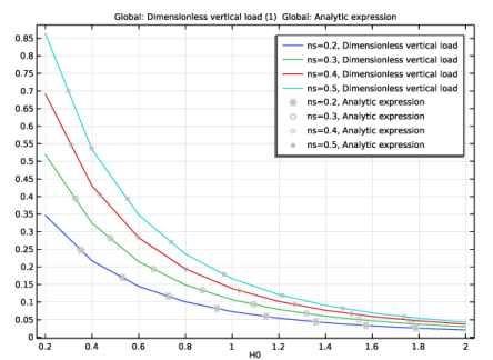
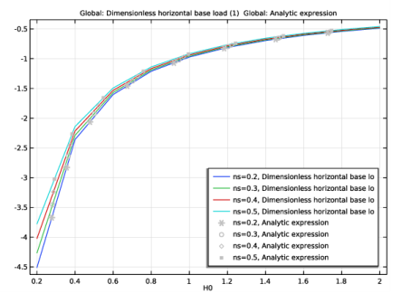
The results of the simulation are compared with the analytic expressions discussed above in Figure 2 to Figure 7. In all cases the agreement between COMSOL and the analytic results is excellent. The ratio H0 = h0/sh is a measure of the step height relative to the outlet height — for smaller values of H0 the step height is greater in relation to the exit height of the bearing. These results show a trend of increasing load bearing capacity with reduced H0 and increased ns, with a corresponding increase in the maximum pressure in the bearing. As discussed in Ref. 1, there is, in fact, an optimum value of H0 and ns, but this optimum occurs at larger values of ns. The flow rate of gas through the bearing increases with increasing H0 as the flow tends toward a pure Couette flow, which produces no back pressure.

Figure 2: Non-dimensional pressure vs distance along the bearing, plotted for different values of the film thickness ratio, H0=h0/sh The computed results are shown as the continuous curves and the theoretical results as the gray symbols.

Figure 3: Non-dimensional maximum pressure vs film thickness ratio, H0=h0/sh. The computed results are shown as the continuous curve and the theoretical result as gray symbols. Different values of the step location ns =Ls/L are shown.

Figure 4: Non-dimensional flow rate vs film thickness ratio, H0=h0/sh. The computed results are shown as the continuous curve and the theoretical result as gray symbols.Different values of the step location ns =Ls/L are shown.

Figure 5: Non-dimensional vertical load vs film thickness ratio, H0=h0/sh. The computed results are shown as the continuous curve and the theoretical result as gray symbols. Different values of the step location ns =Ls/L are shown.

Figure 6: Non-dimensional horizontal wall load vs film thickness ratio, H0=h0/sh. The computed results are shown as the continuous curve and the theoretical result as gray symbols. Different values of the step location ns =Ls/L are shown.

Figure 7: Non-dimensional horizontal base load vs film thickness ratio, H0=h0/sh. The computed results are shown as the continuous curve and the theoretical result as gray symbols. Different values of the step location ns =Ls/L are shown.

Reference

1. B.J. Hamrock, S.R. Schmid, and B.O. Jacobson, Fundamentals of Fluid Film Lubrication, Marcel Dekker, New York, 2004.

This model is based on the discussion entitled Parallel-Step Slider Bearing in section 8.6 of the above reference.

CFD_Module/Thin-Film_Flow/step_bearing_1d

Modeling Instructions

From the menu, choose .

New

In the window, click

Model Wizard

In the window, click

In the tree, select .

Click .

Click

In the tree, select .

Click

Global Definitions

Parameters 1

In the window, under click .

In the window for , locate the section.

In the table, enter the following settings:


Name	Expression	Value	Description
L	1[mm]	0.001 m	Bearing length
H0	0.1	0.1	Dimensionless height at end
sh	2[um]	2E-6 m	Additional height at start
h0	sh*H0	2E-7 m	Height at end
ns	0.6	0.6	Dimensionless step location
Ls	L*ns	6E-4 m	Step x-coordinate
Vb	0.1[mm/s]	1E-4 m/s	Velocity of base
mu0	0.8[Pa*s]	0.8 Pa·s	Fluid viscosity
rho0	900[kg/m^3]	900 kg/m³	Fluid density

Geometry 1

Polygon 1 (pol1)

In the toolbar, click

In the window for , locate the section.

From the list, choose .

Locate the section. From the list, choose .

In the text field, type 0 L Ls.

In the text field, type 0 0 0.

Click

Definitions

Integration 1 (intop1)

In the toolbar, click

and choose .

In the window for , locate the section.

From the list, choose .

Click in the window and then press Ctrl+A to select both boundaries.

Integration 2 (intop2)

In the toolbar, click

and choose .

In the window for , locate the section.

From the list, choose .

Select Point 1 only.

Variables 1

In the toolbar, click

In the window for , locate the section.

In the table, enter the following settings:


Name	Expression	Unit	Description
Xd	x/L		Dimensionless length
Pd	pfilmsh^2/(mu0Vb*L)		Dimensionless pressure
Qd	2intop2(tff.vavextff.h)/(sh*Vb)		Dimensionless flow rate
VLd	-intop1(tff.fwally)sh^2/(mu0Vb*L^2)		Dimensionless vertical load
HLwd	intop1(tff.fwallx)sh/(mu0Vb*L)		Dimensionless horizontal wall load
HLbd	intop1(tff.fbasex)sh/(mu0Vb*L)		Dimensionless horizontal base load
Pmaxan	6ns(1-ns)/((1-ns)(H0+1)^3+nsH0^3)		Analytic dimensionless maximum pressure
Qan	-Pmaxan(H0+1)^3/(6ns)+H0+1		Analytic dimensionless flow rate
VLan	Pmaxan/2		Analytic dimensionless vertical load
HLwan	-Pmaxan/2+(H0+1-ns)/(H0*(1+H0))		Analytic dimensionless horizontal load, wall
HLban	-Pmaxan/2-(H0+1-ns)/(H0*(1+H0))		Analytic dimensionless horizontal load, base