PDF

Pipe Erosion due to Contaminant Particles
Introduction
Pipelines used to transport fluids such as oil and gas often contain solid contaminant particles, such as sand, that are carried along with the moving fluid. These solid particles can impinge on the pipe walls, deforming or stripping away the surface material in a process known as erosion.
In addition to physical depletion of material from the pipe walls, erosion by solid particles may be detrimental to the condition of the pipelines in other, more indirect ways. For example, solid particles may damage corrosion-resistant layers inside the pipes or remove chemical inhibitors from the interior surfaces, exposing material in the pipe walls that may be more susceptible to corrosion. Such synergistic effects, often indicated by the term erosion-corrosion, can be extremely costly as they may cause oil and gas pipelines to degrade at an accelerated rate.
Simulation of pipeline erosion can be a powerful and cost-effective tool for design, optimization, and diagnostics. In this example, the rate of erosive wear in a 90° pipe elbow is computed and compared for three different erosion models.
Model Definition
The model geometry consists of two straight cylindrical pipe sections, each 50 cm in length and 20 cm in diameter. The straight sections are connected by a 90° pipe bend with a 50 cm radius of curvature. The pipe is used to transport water at room temperature with a maximum inlet velocity of 20 m/s. Only half the pipe is modeled because the xy-plane is a symmetry plane. The water is treated as an incompressible fluid.
The pipe also transports solid particles at a rate of 0.6 kg/h. Although such particles would typically be assigned a size distribution, in this tutorial all particles have equal diameters of 0.17 mm.
Modeling Considerations
The high Reynolds number, ReD = 3.96 × 106 based on the pipe diameter, calls for a turbulence model with wall functions. Here, the k-ω turbulence model is selected over the k-ε model because it is more accurate than the k-ε model for flows involving strong streamline curvature (Ref. 2).
A structured mesh is used to reduce the computational cost of the model. The boundary layer mesh is used to ensure that the flow close to the pipe walls is adequately resolved.
Results and Discussion
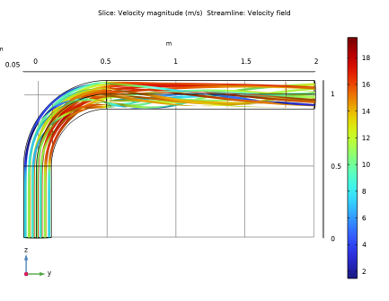
The resulting velocity distribution is shown in Figure 1. There is a separation zone after the bend which is consistent with the results in Ref. 1. The outlet pipe length was made longer than the inlet pipe length in order to resolve this region. Figure 2 shows a contour plot of the corresponding pressure distribution. The wall resolution in viscous units is plotted in Figure 3; the value is less than 100 everywhere, suggesting that the boundary mesh on the walls is adequately refined.
The particle trajectories are shown in Figure 4. The Disappear Wall condition has been used to hide particles that move through the pipe bend without touching the walls, so only the particles that have made contact with surfaces of the pipe bend are shown. The color expression is the acute angle of incidence in degrees, measured from the surface normal. It is clear that the particles only strike the surface at grazing angles.
Three different erosion models are used to compute the rate of erosive wear on the surface of the pipe elbow: Finnie, DNV, and E/CRC. These erosion models are built into the dedicated Erosion node, which can be added as a subnode to any Wall boundary condition. It is possible to solve for the rate of erosive wear using several different erosion models on the same set of boundaries. The erosion models are described in greater detail in the Particle Tracing Module User’s Guide.
Figure 1: Velocity streamlines in the pipe elbow.
Figure 2: Contour plot of pressure in the pipe elbow.
Figure 3: Wall resolution in viscous units. A value greater than several hundreds usually indicates that a mesh needs to be refined in the wall normal direction.
Figure 4: Particle trajectories. The color expression is the acute angle of incidence, measured from the surface normal.
Figure 5: Rate of erosive wear on the pipe walls, computed using the Finnie model.
Figure 6: Rate of erosive wear on the pipe walls, computed using the DNV model.
Figure 7: Rate of erosive wear on the pipe walls, computed using the E/CRC model.
References
1. G.F. Homicz, “Computational Fluid Dynamic Simulations of Pipe Elbow Flow,” SAND REPORT, SAND2004-3467, Sandia National Laboratories, 2004.
2. F. Menter, “Zonal Two Equation k-ω Turbulence Models for Aerodynamic Flows,” AIAA Paper #93-2906, 24th Fluid Dynamics Conference, July 1993.
Application Library path: CFD_Module/Particle_Tracing/pipe_elbow_erosion
Modeling Instructions
From the File menu, choose New.
New
In the New window, click  Model Wizard.
Model Wizard
1
In the Model Wizard window, click  3D.
2
In the Select Physics tree, select Fluid Flow>Single-Phase Flow>Turbulent Flow>Turbulent Flow, k-ω (spf).
3
Click Add.
4
Click  Study.
5
In the Select Study tree, select General Studies>Stationary.
6
Global Definitions
Parameters 1
Load the model’s parameters from a text file.
1
In the Model Builder window, under Global Definitions click Parameters 1.
2
In the Settings window for Parameters, locate the Parameters section.
3
Click  Load from File.
4
Geometry 1
The geometry consists of two straight cylindrical pipe sections connected by a 90 degree pipe elbow.
Cylinder 1 (cyl1)
1
In the Geometry toolbar, click  Cylinder.
2
In the Settings window for Cylinder, locate the Size and Shape section.
3
In the Radius text field, type r1.
4
In the Height text field, type L1.
Torus 1 (tor1)
1
In the Geometry toolbar, click  Torus.
2
In the Settings window for Torus, locate the Size and Shape section.
3
In the Major radius text field, type R3.
4
In the Minor radius text field, type r3.
5
In the Revolution angle text field, type 90.
6
Locate the Position section. In the y text field, type R3.
7
In the z text field, type L1.
8
Locate the Axis section. From the Axis type list, choose x-axis.
9
Locate the Rotation Angle section. In the Rotation text field, type 180.
Cylinder 2 (cyl2)
1
In the Geometry toolbar, click  Cylinder.
2
In the Settings window for Cylinder, locate the Size and Shape section.
3
In the Radius text field, type r2.
4
In the Height text field, type L2.
5
Locate the Position section. In the y text field, type R3.
6
In the z text field, type L1+R3.
7
Locate the Axis section. From the Axis type list, choose y-axis.
Use a work plane to create a separate boundary where particles will be released at the pipe inlet.
Work Plane 1 (wp1)
1
In the Geometry toolbar, click  Work Plane.
2
In the Settings window for Work Plane, locate the Plane Definition section.
3
From the Plane type list, choose Face parallel.
4
On the object cyl1, select Boundary 3 only.
It might be easier to select the correct boundary by using the Selection List window. To open this window, in the Home toolbar click Windows and choose Selection List. (If you are running the cross-platform desktop, you find Windows in the main menu.)
5
Click  Show Work Plane.
Work Plane 1 (wp1)>Plane Geometry
1
In the Settings window for Plane Geometry, locate the Visualization section.
2
Select the View work plane geometry in 3D check box.
Work Plane 1 (wp1)>Circle 1 (c1)
1
In the Work Plane toolbar, click  Circle.
2
In the Settings window for Circle, locate the Size and Shape section.
3
In the Radius text field, type 0.05.
Union 1 (uni1)
1
In the Model Builder window, right-click Geometry 1 and choose Booleans and Partitions>Union.
2
Click in the Graphics window and then press Ctrl+A to select all objects.
To save time and memory, exploit symmetry by only modeling the fluid flow and particle motion in half of the geometry.
Work Plane 2 (wp2)
1
In the Geometry toolbar, click  Work Plane.
2
In the Settings window for Work Plane, locate the Plane Definition section.
3
From the Plane list, choose yz-plane.
Partition Objects 1 (par1)
1
In the Geometry toolbar, click  Booleans and Partitions and choose Partition Objects.
2
3
In the Settings window for Partition Objects, locate the Partition Objects section.
4
From the Partition with list, choose Work plane.
Delete Entities 1 (del1)
1
Right-click Geometry 1 and choose Delete Entities.
2
In the Settings window for Delete Entities, locate the Entities or Objects to Delete section.
3
From the Geometric entity level list, choose Domain.
4
On the object par1, select Domains 1–3 only.
5
Click  Build All Objects.
6
Click the  Zoom Extents button in the Graphics toolbar.
Turbulent Flow, k-ω (spf)
Inlet 1
1
In the Model Builder window, under Component 1 (comp1) right-click Turbulent Flow, k-ω (spf) and choose Inlet.
2
3
In the Settings window for Inlet, locate the Boundary Condition section.
4
From the list, choose Fully developed flow.
5
Locate the Fully Developed Flow section. In the Uav text field, type Vi.
6
In the Model Builder window, click Turbulent Flow, k-ω (spf).
7
In the Settings window for Turbulent Flow, k-ω, locate the Turbulence section.
8
From the Wall treatment list, choose Wall functions.
Outlet 1
1
In the Physics toolbar, click  Boundaries and choose Outlet.
2
Symmetry 1
1
In the Physics toolbar, click  Boundaries and choose Symmetry.
2
Add Material
1
In the Home toolbar, click  Add Material to open the Add Material window.
2
Go to the Add Material window.
3
In the tree, select Built-in>Water, liquid.
4
Click Add to Component in the window toolbar.
5
In the Home toolbar, click  Add Material to close the Add Material window.
Mesh 1
Boundary Layers 1
In the Mesh toolbar, click  Boundary Layers.
Boundary Layer Properties
1
In the Model Builder window, click Boundary Layer Properties.
2
In the Settings window for Boundary Layer Properties, locate the Layers section.
3
In the Number of layers text field, type 5.
4
In the Stretching factor text field, type 2.2.
5
In the Thickness adjustment factor text field, type 0.4.
Size
1
In the Model Builder window, under Component 1 (comp1)>Mesh 1 click Size.
2
In the Settings window for Size, locate the Element Size section.
3
From the Calibrate for list, choose Fluid dynamics.
4
From the Predefined list, choose Extra fine.
5
Click to expand the Element Size Parameters section. In the Maximum element size text field, type r3/10.
Boundary Layers 1
1
In the Model Builder window, click Boundary Layers 1.
2
In the Settings window for Boundary Layers, locate the Geometric Entity Selection section.
3
From the Geometric entity level list, choose Boundary.
4
5
Click to expand the Transition section. Clear the Smooth transition to interior mesh check box.
Boundary Layer Properties
1
In the Model Builder window, click Boundary Layer Properties.
2
Swept 1
In the Mesh toolbar, click  Swept.
Distribution 1
1
Right-click Swept 1 and choose Distribution.
2
In the Settings window for Distribution, locate the Domain Selection section.
3
Click  Clear Selection.
4
5
Locate the Distribution section. In the Number of elements text field, type 40.
Distribution 2
1
In the Model Builder window, right-click Swept 1 and choose Distribution.
2
In the Settings window for Distribution, locate the Domain Selection section.
3
Click  Clear Selection.
4
5
Locate the Distribution section. In the Number of elements text field, type 80.
Distribution 3
1
Right-click Swept 1 and choose Distribution.
2
In the Settings window for Distribution, locate the Domain Selection section.
3
Click  Clear Selection.
4
5
Locate the Distribution section. From the Distribution type list, choose Predefined.
6
In the Number of elements text field, type 70.
7
In the Element ratio text field, type 5.
8
From the Growth rate list, choose Exponential.
9
Click  Build All.
Study 1
In the Home toolbar, click  Compute.
Results
Slice
1
In the Model Builder window, expand the Velocity (spf) node, then click Slice.
2
In the Settings window for Slice, locate the Plane Data section.
3
From the Plane list, choose zx-planes.
Streamline 1
1
In the Model Builder window, right-click Velocity (spf) and choose Streamline.
2
In the Settings window for Streamline, locate the Coloring and Style section.
3
Find the Line style subsection. From the Type list, choose Ribbon.
4
Color Expression 1
1
In the Velocity (spf) toolbar, click  Color Expression.
2
In the Settings window for Color Expression, locate the Coloring and Style section.
3
Clear the Color legend check box.
4
In the Velocity (spf) toolbar, click  Plot.
5
Click the  Go to YZ View button in the Graphics toolbar.
Compare the resulting plot to Figure 1.
Pressure (spf)
1
In the Model Builder window, under Results click Pressure (spf).
2
In the Pressure (spf) toolbar, click  Plot.
Compare the resulting plot to Figure 2.
Wall Resolution (spf)
1
In the Model Builder window, click Wall Resolution (spf).
2
In the Wall Resolution (spf) toolbar, click  Plot.
The Wall Resolution plot is used to verify that the mesh resolution in the model is adequate. Compare the resulting plot to Figure 3.
Add Physics
1
In the Home toolbar, click  Add Physics to open the Add Physics window.
2
Go to the Add Physics window.
3
In the tree, select Fluid Flow>Particle Tracing>Particle Tracing for Fluid Flow (fpt).
4
Find the Physics interfaces in study subsection. Clear the check box next to Study 1.
5
Click Add to Component 1 in the window toolbar.
6
In the Home toolbar, click  Add Physics to close the Add Physics window.
Particle Tracing for Fluid Flow (fpt)
When Specify mass flow rate is selected from the Particle release specification list, each model particle is assumed to represent a number of real particles per unit time. Thus it is possible to compute the rate of erosive wear by contaminant particles in a stationary flow field.
1
In the Settings window for Particle Tracing for Fluid Flow, locate the Particle Release and Propagation section.
2
From the Particle release specification list, choose Specify mass flow rate.
Inlet 1
1
Right-click Component 1 (comp1)>Particle Tracing for Fluid Flow (fpt) and choose Inlet.
2
In the Mass flow rate text field, type 0.6[kg/h].
3
In the Settings window for Inlet, locate the Initial Position section.
4
From the Initial position list, choose Density.
5
In the N text field, type 5000.
6
In the ρ text field, type spf.U.
7
Locate the Initial Velocity section. From the u list, choose Velocity field (spf).
8
Particle Properties 1
1
In the Model Builder window, click Particle Properties 1.
2
In the Settings window for Particle Properties, locate the Particle Properties section.
3
From the ρp list, choose User defined. In the associated text field, type sigma.
4
In the dp text field, type 1.7E-4[m].
Compute the rate of erosive wear at the pipe elbow using three different erosion models.
Wall 1
In the Model Builder window, click Wall 1.
Erosion 1
1
In the Physics toolbar, click  Attributes and choose Erosion.
2
In the Settings window for Erosion, locate the Erosion Model section.
3
In the ci text field, type fc.
4
In the K text field, type kappa.
5
In the HV text field, type Hs.
6
In the ρ text field, type rho.
Wall 1
In the Model Builder window, click Wall 1.
Erosion 2
1
In the Physics toolbar, click  Attributes and choose Erosion.
2
In the Settings window for Erosion, locate the Erosion Model section.
3
From the Erosion model list, choose DNV.
Wall 1
In the Model Builder window, click Wall 1.
Erosion 3
1
In the Physics toolbar, click  Attributes and choose Erosion.
2
In the Settings window for Erosion, locate the Erosion Model section.
3
From the Erosion model list, choose E/CRC.
Drag Force 1
1
In the Physics toolbar, click  Domains and choose Drag Force.
2
In the Settings window for Drag Force, locate the Domain Selection section.
3
From the Selection list, choose All domains.
4
Locate the Drag Force section. From the u list, choose Velocity field (spf).
Select an option from the Turbulent dispersion model list to apply a random perturbation term to the fluid velocity when computing the drag force.
5
Locate the Turbulent Dispersion section. From the Turbulent dispersion model list, choose Discrete random walk.
6
From the k list, choose Turbulent kinetic energy (spf).
7
From the ε list, choose Turbulent dissipation rate (spf/fp1).
Wall 2
1
In the Physics toolbar, click  Boundaries and choose Wall.
2
Symmetry 1
1
In the Physics toolbar, click  Boundaries and choose Symmetry.
2
Outlet 1
1
In the Physics toolbar, click  Boundaries and choose Outlet.
2
Apply the Disappear Wall condition at the outlet to avoid rendering particles that pass through the pipe elbow without hitting the walls.
3
In the Settings window for Outlet, locate the Outlet section.
4
From the Wall condition list, choose Disappear.
Add Study
1
In the Home toolbar, click  Add Study to open the Add Study window.
2
Go to the Add Study window.
3
Find the Studies subsection. In the Select Study tree, select General Studies>Time Dependent.
4
Click Add Study in the window toolbar.
5
In the Home toolbar, click  Add Study to close the Add Study window.
Study 2
Step 1: Time Dependent
1
In the Settings window for Time Dependent, locate the Study Settings section.
2
In the Output times text field, type range(0,5e-3,0.12).
3
From the Tolerance list, choose User controlled.
4
In the Relative tolerance text field, type 1e-2.
5
Locate the Physics and Variables Selection section. In the table, clear the Solve for check box for Turbulent Flow, k-ω (spf).
6
Click to expand the Values of Dependent Variables section. Find the Values of variables not solved for subsection. From the Settings list, choose User controlled.
7
From the Method list, choose Solution.
8
From the Study list, choose Study 1, Stationary.
9
In the Home toolbar, click  Compute.
Results
Particle Trajectories (fpt)
In the Model Builder window, expand the Particle Trajectories (fpt) node.
Color Expression 1
1
In the Model Builder window, expand the Results>Particle Trajectories (fpt)>Particle Trajectories 1 node, then click Color Expression 1.
2
In the Settings window for Color Expression, click Replace Expression in the upper-right corner of the Expression section. From the menu, choose Component 1 (comp1)>Particle Tracing for Fluid Flow>Particle properties>fpt.phii - Acute angle of incidence - rad.
3
Locate the Expression section. From the Unit list, choose °.
4
In the Particle Trajectories (fpt) toolbar, click  Plot.
Compare the resulting plot to Figure 4.
Create a Mirror dataset to visualize the rate of erosive wear on the surface.
Mirror 3D 1
1
In the Results toolbar, click  More Datasets and choose Mirror 3D.
2
In the Settings window for Mirror 3D, locate the Data section.
3
From the Dataset list, choose Study 2/Solution 2 (sol2).
Erosion rate, Finnie
1
In the Model Builder window, under Results click Accumulated Variable (fpt).
2
In the Settings window for 3D Plot Group, type Erosion rate, Finnie in the Label text field.
3
Locate the Data section. From the Dataset list, choose Mirror 3D 1.
Surface 1
1
In the Model Builder window, expand the Erosion rate, Finnie node, then click Surface 1.
2
In the Settings window for Surface, click to expand the Quality section.
3
From the Smoothing list, choose Everywhere.
4
In the Erosion rate, Finnie toolbar, click  Plot.
5
Click the  Zoom Extents button in the Graphics toolbar.
Compare the resulting plot to Figure 5.
Erosion rate, DNV
1
In the Model Builder window, right-click Erosion rate, Finnie and choose Duplicate.
2
In the Settings window for 3D Plot Group, type Erosion rate, DNV in the Label text field.
Surface 1
1
In the Model Builder window, expand the Erosion rate, DNV node, then click Surface 1.
2
In the Settings window for Surface, locate the Expression section.
3
In the Expression text field, type fpt.wall1.ero2.EM.
4
In the Erosion rate, DNV toolbar, click  Plot.
Compare the resulting plot to Figure 6.
Erosion rate, E/CRC
1
In the Model Builder window, right-click Erosion rate, DNV and choose Duplicate.
2
In the Settings window for 3D Plot Group, type Erosion rate, E/CRC in the Label text field.
Surface 1
1
In the Model Builder window, expand the Erosion rate, E/CRC node, then click Surface 1.
2
In the Settings window for Surface, locate the Expression section.
3
In the Expression text field, type fpt.wall1.ero3.EM.
4
In the Erosion rate, E/CRC toolbar, click  Plot.
Compare the resulting plot to Figure 7.