PDF

Stationary Incompressible Flow over a Backstep
Introduction
This tutorial model solves the incompressible Navier-Stokes equations in a backstep geometry. A characteristic feature of fluid flow in geometries of this kind is the recirculation region that forms where the flow exits the narrow inlet region. The model clearly demonstrates the formation of such a region, which is best displayed by visualizing the flow streamlines.
Model Definition
Model Geometry
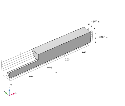
The model consists of a pipe connected to a block-shaped tank; see Figure 1. Due to symmetry, it is sufficient to model one eighth of the full geometry. The pipe has an inlet at one end, and the tank has an outlet at the opposite end. All other boundaries are solid walls.
Figure 1: Model geometry.
Domain Equation and Boundary Conditions
The flow in this model is laminar, so a Laminar Flow interface will be used. The inlet flow is fully developed, which will be specified by the corresponding inlet boundary condition. This boundary condition computes the flow profile for fully developed flow in a channel of arbitrary cross section. The boundary condition at the outlet sets a constant relative pressure. Furthermore, the vertical and inclined boundaries along the length of the geometry are symmetry boundaries. All other boundaries are solid walls described by a no slip boundary condition.
Results
Figure 2 shows a combined surface and arrow plot of the flow velocity. This plot does not reveal the recirculation region in the tank immediately beyond the inlet pipe’s end. For this purpose, a streamline plot is more useful, as demonstrated in Figure 3.
Figure 2: The velocity field in the backstep geometry.
Figure 3: The recirculation region visualized using a velocity streamline plot.
Application Library path: CFD_Module/Single-Phase_Flow/backstep
Modeling Instructions
From the File menu, choose New.
New
In the New window, click  Model Wizard.
Model Wizard
1
In the Model Wizard window, click  3D.
2
In the Select Physics tree, select Fluid Flow>Single-Phase Flow>Laminar Flow (spf).
3
Click Add.
4
Click  Study.
5
In the Select Study tree, select General Studies>Stationary.
6
Global Definitions
Parameters 1
1
In the Model Builder window, under Global Definitions click Parameters 1.
2
In the Settings window for Parameters, locate the Parameters section.
3
Geometry 1
You can build the backstep geometry from geometric primitives. Here, instead, use a file containing the sequence of geometry features that has been provided for convenience.
1
In the Geometry toolbar, click Insert Sequence and choose Insert Sequence.
2
3
In the Geometry toolbar, click  Build All.
4
Click the  Zoom Extents button in the Graphics toolbar.
The model geometry is now complete (Figure 1).
Add Material
1
In the Home toolbar, click  Add Material to open the Add Material window.
2
Go to the Add Material window.
3
In the tree, select Built-in>Water, liquid.
4
Click Add to Component in the window toolbar.
5
In the Home toolbar, click  Add Material to close the Add Material window.
Laminar Flow (spf)
Inlet 1
1
In the Model Builder window, under Component 1 (comp1) right-click Laminar Flow (spf) and choose Inlet.
2
3
In the Settings window for Inlet, locate the Boundary Condition section.
4
From the list, choose Fully developed flow.
5
Locate the Fully Developed Flow section. In the Uav text field, type v0.
Symmetry 1
1
In the Physics toolbar, click  Boundaries and choose Symmetry.
2
Outlet 1
1
In the Physics toolbar, click  Boundaries and choose Outlet.
2
3
In the Settings window for Outlet, locate the Pressure Conditions section.
4
Select the Normal flow check box.
Mesh 1
1
In the Model Builder window, under Component 1 (comp1) click Mesh 1.
2
In the Settings window for Mesh, locate the Physics-Controlled Mesh section.
3
From the Element size list, choose Coarse.
4
Click  Build All.
5
Click the  Zoom Extents button in the Graphics toolbar.
Study 1
In the Home toolbar, click  Compute.
Results
A slice plot of the velocity and a plot showing the pressure distribution on the exterior walls are produced automatically. Change the slice plot to get Figure 2.
Slice
1
In the Model Builder window, expand the Velocity (spf) node.
2
Right-click Results>Velocity (spf)>Slice and choose Delete. Click Yes to confirm.
Surface 1
In the Model Builder window, right-click Velocity (spf) and choose Surface.
Arrow Surface 1
1
Right-click Velocity (spf) and choose Arrow Surface.
2
In the Settings window for Arrow Surface, locate the Coloring and Style section.
3
From the Arrow length list, choose Logarithmic.
4
From the Color list, choose Yellow.
5
Click the  Zoom Extents button in the Graphics toolbar.
6
In the Velocity (spf) toolbar, click  Plot.
To see the recirculation effects, create a streamline plot of the velocity field.
Velocity, Streamlines
1
In the Home toolbar, click  Add Plot Group and choose 3D Plot Group.
2
In the Settings window for 3D Plot Group, type Velocity, Streamlines in the Label text field.
Streamline 1
1
Right-click Velocity, Streamlines and choose Streamline.
2
3
In the Settings window for Streamline, locate the Coloring and Style section.
4
Find the Line style subsection. From the Type list, choose Tube.
Color Expression 1
Right-click Streamline 1 and choose Color Expression.