
|
|
|
|
1
|
|
2
|
In the Select Physics tree, select Fluid Flow>Single-Phase Flow>Turbulent Flow>Turbulent Flow, k-ω (spf).
|
|
3
|
Click Add.
|
|
4
|
Click
|
|
5
|
|
6
|
Click
|
|
1
|
|
2
|
|
3
|
|
4
|
Browse to the model’s Application Libraries folder and double-click the file air_filter_parameters_1.txt.
|
|
1
|
|
2
|
|
3
|
|
4
|
Browse to the model’s Application Libraries folder and double-click the file air_filter_parameters_2.txt.
|
|
1
|
|
2
|
|
3
|
|
1
|
|
2
|
|
3
|
|
1
|
|
2
|
|
3
|
|
4
|
|
5
|
|
6
|
|
7
|
|
8
|
Locate the Selections of Resulting Entities section. Find the Cumulative selection subsection. Click New.
|
|
9
|
|
10
|
Click OK.
|
|
1
|
|
2
|
|
3
|
|
1
|
|
2
|
|
3
|
|
4
|
|
5
|
|
6
|
|
7
|
Locate the Selections of Resulting Entities section. Find the Cumulative selection subsection. From the Contribute to list, choose Inner Grill.
|
|
8
|
|
1
|
|
2
|
|
3
|
|
4
|
|
5
|
|
6
|
|
7
|
|
1
|
|
2
|
|
3
|
|
4
|
|
1
|
|
2
|
Select the object r2 only.
|
|
3
|
|
4
|
|
5
|
Locate the Selections of Resulting Entities section. Find the Cumulative selection subsection. From the Contribute to list, choose Inner Grill.
|
|
1
|
|
2
|
|
4
|
Locate the Selections of Resulting Entities section. Select the Resulting objects selection check box.
|
|
5
|
|
6
|
From the Color list, choose None or — if you are running the cross-platform desktop —Custom. On the cross-platform desktop, click the Color button.
|
|
7
|
Click Define custom colors.
|
|
9
|
Click Add to custom colors.
|
|
10
|
|
11
|
|
12
|
|
13
|
Click OK.
|
|
1
|
|
2
|
|
3
|
|
4
|
|
5
|
|
6
|
|
7
|
Locate the Selections of Resulting Entities section. Select the Resulting objects selection check box.
|
|
8
|
|
9
|
|
10
|
|
11
|
Click OK.
|
|
1
|
|
2
|
|
3
|
|
4
|
Select the Transparency check box.
|
|
1
|
|
2
|
|
1
|
|
2
|
|
3
|
|
4
|
|
5
|
|
6
|
|
7
|
Locate the Selections of Resulting Entities section. Find the Cumulative selection subsection. Click New.
|
|
8
|
|
9
|
Click OK.
|
|
1
|
|
2
|
|
3
|
|
4
|
|
5
|
|
6
|
|
7
|
Locate the Selections of Resulting Entities section. Find the Cumulative selection subsection. Click New.
|
|
8
|
|
9
|
Click OK.
|
|
1
|
|
2
|
|
3
|
|
4
|
|
5
|
|
6
|
Locate the Selections of Resulting Entities section. Find the Cumulative selection subsection. Click New.
|
|
7
|
|
8
|
Click OK.
|
|
1
|
|
2
|
|
3
|
|
4
|
|
1
|
|
2
|
On the object fin, select Domains 1 and 5 only.
|
|
3
|
|
4
|
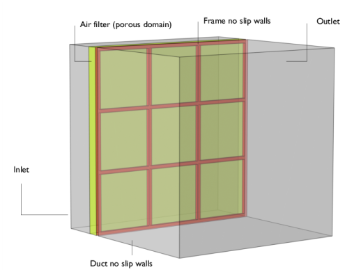
Adjust camera to reproduce Figure 1.
|
|
1
|
|
2
|
|
3
|
In the tree, select Built-in>Air.
|
|
4
|
|
5
|
|
1
|
|
2
|
|
3
|
|
4
|
|
5
|
Locate the Material Properties section. In the Material properties tree, select Basic Properties>Porosity.
|
|
6
|
|
7
|
|
1
|
|
2
|
|
3
|
|
4
|
|
5
|
|
6
|
Click OK.
|
|
1
|
|
2
|
|
3
|
|
4
|
|
5
|
|
6
|
Click OK.
|
|
1
|
|
2
|
|
3
|
|
1
|
|
2
|
|
3
|
|
1
|
|
2
|
|
3
|
|
1
|
|
3
|
|
4
|
|
1
|
|
1
|
|
2
|
|
3
|
|
4
|
|
1
|
|
2
|
|
3
|
|
4
|
|
5
|
|
1
|
|
2
|
|
3
|
|
4
|
|
1
|
|
2
|
|
3
|
|
4
|
|
6
|
|
7
|
|
1
|
|
2
|
|
3
|
|
5
|
|
6
|
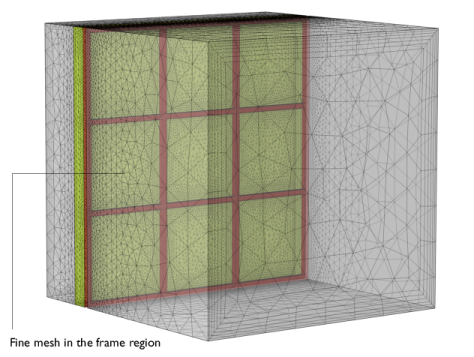
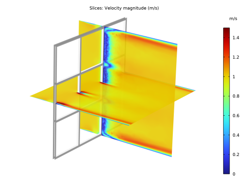
Reproduce Figure 2.
|
|
1
|
|
2
|
|
3
|
|
4
|
|
5
|
|
6
|
|
1
|
|
2
|
|
3
|
|
4
|
|
5
|
|
6
|
|
1
|
|
2
|
|
3
|
|
1
|
|
2
|
|
3
|
|
1
|
|
2
|
|
3
|
|
4
|
|
1
|
|
2
|
|
3
|
|
4
|
|
5
|
Click OK.
|
|
1
|
|
2
|
|
3
|
|
1
|
|
2
|
|
3
|
|
4
|
|
5
|
|
6
|
Locate the Coloring and Style section. Find the Line style subsection. From the Type list, choose Ribbon.
|
|
7
|
|
1
|
|
2
|
|
3
|
|
4
|
|
5
|
|
6
|
|
7
|
Click OK.
|
|
8
|
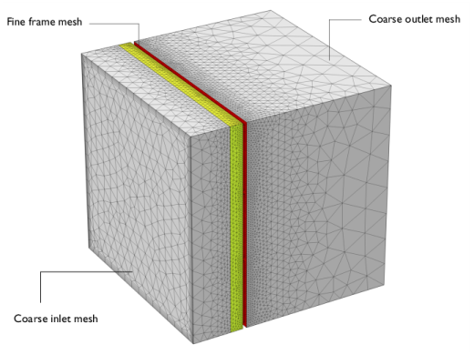
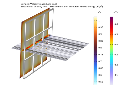
Adjust camera to reproduce Figure 4.
|
|
1
|
|
2
|
In the Settings window for 3D Plot Group, type Velocity and turbulence kinetic energy in the Label text field.
|
|
3
|
|
1
|
In the Model Builder window, expand the Results>Velocity and turbulence kinetic energy>Streamline 1 node, then click Color Expression 1.
|
|
2
|
|
3
|
|
4
|
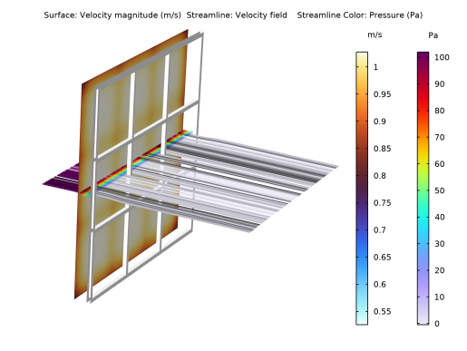
Reproduce Figure 5.
|
|
1
|
In the Model Builder window, right-click Velocity and turbulence kinetic energy and choose Duplicate.
|
|
2
|
|
3
|
|
4
|
|
1
|
|
2
|
|
3
|
Select the Transparency check box.
|
|
4
|
|
1
|
In the Model Builder window, under Results>Velocity slices xy and xz, Ctrl-click to select Surface 2 and Streamline 1.
|
|
2
|
Right-click and choose Delete.
|
|
1
|
|
2
|
|
3
|
|
4
|
|
5
|
|
6
|
|
7
|
|
8
|
|
9
|
|
1
|
|
2
|
|
3
|
|
4
|
|
5
|
|
6
|
|
7
|
|
8
|
Adjust camera to reproduce Figure 6.
|
|
1
|
|
2
|
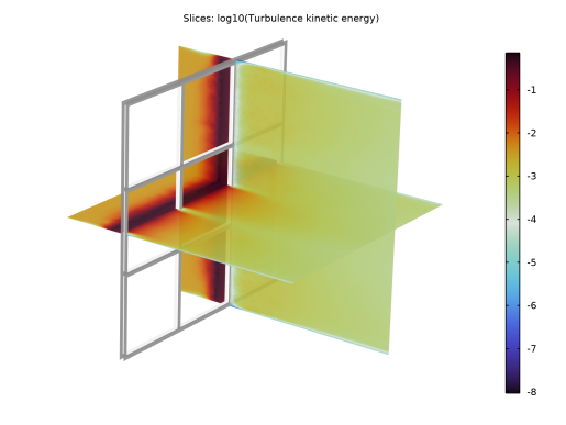
In the Settings window for 3D Plot Group, type log10(Turbulence kinetic energy) slices xy and xz in the Label text field.
|
|
1
|
In the Model Builder window, expand the log10(Turbulence kinetic energy) slices xy and xz node, then click Slice 1.
|
|
2
|
|
3
|
|
4
|
|
5
|
|
6
|
|
7
|
|
8
|
Click OK.
|
|
1
|
|
2
|
|
3
|
|
4
|
Reproduce Figure 7.
|
|
1
|
|
2
|
|
3
|
|
4
|
|
5
|
|
6
|
|
7
|
|
8
|
|
1
|
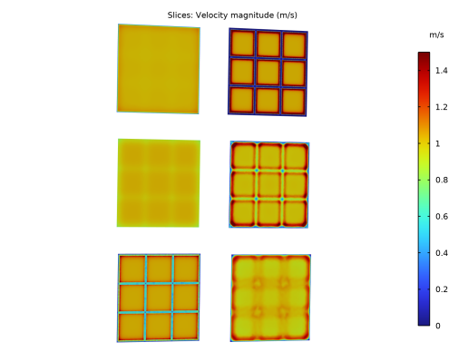
In the Model Builder window, under Results>Velocity slices yz planes, Ctrl-click to select Surface 1 and Slice 2.
|
|
2
|
Right-click and choose Delete.
|
|
1
|
|
2
|
|
3
|
|
4
|
|
5
|
|
6
|
|
1
|
|
2
|
|
3
|
|
4
|
|
5
|
|
6
|
|
1
|
|
2
|
|
3
|
|
4
|
|
1
|
|
2
|
|
3
|
|
4
|
|
5
|
|
1
|
|
2
|
|
3
|
|
4
|
|
1
|
|
2
|
|
3
|
|
4
|
|
5
|
Adjust camera to reproduce Figure 8.
|
|
1
|
|
2
|
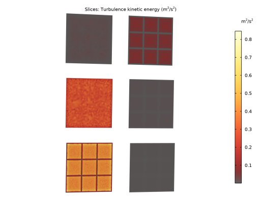
In the Settings window for 3D Plot Group, type Turbulence kinetic energy yz planes in the Label text field.
|
|
1
|
In the Model Builder window, expand the Turbulence kinetic energy yz planes node, then click Slice 1.
|
|
2
|
|
3
|
|
4
|
|
5
|
|
6
|
|
7
|
|
8
|
Click OK.
|
|
1
|
|
2
|
|
3
|
|
1
|
|
2
|
|
3
|
|
1
|
|
2
|
|
3
|
|
1
|
|
2
|
|
3
|
|
1
|
|
2
|
|
3
|
|
4
|
Reproduce Figure 9.
|
|
1
|
|
2
|
|
3
|
|
4
|
|
5
|
|
6
|
|
7
|
|
8
|
|
9
|
|
10
|
|
11
|
|
12
|
Click
|
|
1
|
|
2
|
|
3
|
|
4
|
|
5
|
Click
|