PDF

1D Isothermal Nickel–Metal Hydride Battery
Introduction
This example simulates the discharge of a nickel–metal hydride (Ni–MH) battery using the Battery with Binary Electrolyte interface. The geometry is in one dimension and the model is isothermal. The model serves as an introduction to Ni–MH modeling, and can be further extended to include various side reactions. The model is based on a study by Paxton and Newman (Ref. 1), with updated equilibrium potentials from a more recent study by Albertus and others (Ref. 2).
Figure 1: Cross section of a NiMH battery showing the main electrochemical processes that occur during discharge.
The model includes the following processes:
Model Definition
This example models the battery cross section in 1D, which implies that edge effects in the length and height of the battery are neglected. The example uses the following domains:
The electric potential in the electron conducting phase, , is calculated using a charge balance based on Ohm’s law, where the charge transfer reactions result in source or sink term. For the porous electrodes effective conductivities, σseff, are used that take porosity and tortuosity into account as given by the following expression:
where γ is the Bruggeman coefficient, which is set to 1.5 in this model, corresponding to a packed bed of spherical particles. Also, the diffusion coefficient for the electrolyte salt is corrected for the tortuosity and the porosity in this way.
The ionic charge balances and material balances are modeled according to the equations for a binary 1:1 electrolyte, with both the anion (OH-) and the solvent (H2O) participating in the electrode reactions (Ref. 1).
Fickian diffusion describes the transport in the spherical particles. The diffusion equation is expressed in spherical coordinates for the material balance of intercalated hydrogen atoms in the particles.
Butler-Volmer electrode kinetics describes the local charge transfer current density in the electrodes. The Butler-Volmer expressions are introduced as source or sink terms in the charge balances and material balances.
Boundary Conditions
For the electronic current balance, a potential of 0 V is set on the negative electrode’s current collector/feeder boundary. At the positive electrode current collector/feeder, the current density is specified to a constant discharge current density. The inner boundaries facing the separator are insulating for electric currents.
For the ionic charge balance in the electrolyte, the current collector/feeder boundaries are insulating. Insulating conditions also apply to the material balances.
At the particle surface in the local particle model, the material flux is determined by the local electrochemical reaction rate.
Material Properties
The material properties are those of a typical NiMH. The electrolyte is KOH, diluted in water to a 30% (wt) solution. The active electrode materials are a metal hydride (LaNi5Hx) for the negative electrode and a nickel oxide (NiOHOHy) for the positive electrode.
The equilibrium potential of the negative and positive electrodes are composition dependent through experimentally measured data. This data is tabulated in interpolating functions in the model and the properties vary significantly during charge and discharge due to the changes in composition.
The model uses constant values for the electrolyte conductivity, the electrolyte diffusivity, and the activity variation with concentration in the electrolyte. The activity coefficients are assumed to be constant in the electrode reactions. For more accurate simulations you can use concentration-dependent expressions for these properties (Ref. 1).
Figure 2 displays the equilibrium potentials for the negative and positive electrodes as functions of the measured state of charge (SOC).
Figure 2: The equilibrium voltage of the electrode materials.
The initial concentration values within the electrode particles are set to correspond to a fully charged battery.
For complete details on the material properties and constants, see Ref. 1.
Results and Discussion
Discharge Curves
The battery is initially at a fully charged state, discharge at two different current densities are simulated and displayed here. This model defines end-of-discharge as the time when the cell voltage drops below 0.99 V. The nominal discharge current density, corresponding to case 1C below (a current density corresponding to a theoretical full discharge in one hour), is 430 A/m2.
Figure 3: Discharge curves for various discharge rates.
Figure 3 shows that the maximum discharge capacity of 430 Ah/m2 is obtained for the a current density of 43 A/m2 (0.1 C). It can also be seen that the discharge capacity decreases slightly when applying a 1 C discharge current. At 1 C, the battery delivers approximately 90% of the theoretical capacity before it reaches a cell voltage of 1 V.
At the beginning of the discharge the voltage is higher than what is normally seen in a NiMH battery. The reason for this is the absence of side reactions in the model (Ref. 2). (The high voltage on the positive electrode results in a self discharge process in which oxygen is evolved on the positive electrode and transported over to the negative electrode where it is reduced).
The discharge curves are similar to those presented in Ref. 1, with slight deviation due different sources of experimental data for the equilibrium potentials.
Analysis of voltage losses
It is possible to visualize the contributions of the different losses to the total overpotential. You can compare the contribution from the activation overpotential and the electrolyte potential by plotting the electrolyte potential with a bias of 0.91 V as shown in Figure 4. In this way the two plots are within similar range of potential.
Figure 4: Voltage losses in the battery during discharge.
The overpotential at the positive electrode is the largest contributor to the potential losses during a 1C discharge. The figure does not include the electronic potential profile in the solid phase, but the simulations show that contributions from the ohmic losses in the electronic conductors are negligible.
To further investigate the reason for the steep voltage decrease, you can plot the concentration profile in the electrolyte. Figure 5 depicts the profile at several stages during the discharge of the cell.
Figure 5: Electrolyte-phase concentration profiles at various times.
The concentration gradients are quite low and the cell experiences only minor concentration polarization due to electrolyte transport limitations.
Figure 6 shows that the local current density distribution varies during discharge, Initially it is evenly distributed, but toward the end of the discharge more of the current is produced closer to the current collectors, the effect is more pronounced for the negative electrode.
Figure 6: Local current-density distribution within the battery at various stages during the discharge.
The current density is related to the concentration in the solid phase at the surface of the particles. Figure 7 depicts the distribution of the concentration in the solid-phase particles. At the end of discharge most of the concentration of intercalating material is depleted close to the separator at the negative electrode, this explains the lower current densities in this region of the battery, as was shown in Figure 6.
Figure 7: Concentration distribution of intercalated hydrogen in the solid particles during the discharge phase.
As the surface concentration changes, the equilibrium voltage also varies, causing a lower reaction overpotential and a decrease in the local current density. This effect tends to even out the local charge transfer current density to some extent but results in a larger overall voltage loss in the battery.
The difference between the concentration at the surface and at the center of the particles is small throughout the discharge cycle, indicating that the transport of intercalated material within the active particles is not a limiting factor for the performance of the battery at this discharge current density.
References
1. B. Paxton and J. Newman, “Modeling of Nickel/Metal Hydride Batteries,” J. Electrochem. Soc., vol. 144, no. 11, pp. 3818–3831, 1997.
2. P. Albertus, J. Christensen, and J. Newman, “Modeling Side Reactions and Nonisothermal Effects in Nickel Metal-Hydride Batteries,” J. Electrochem. Soc., vol. 155, no. 1, pp. A48–A60, 2008.
Application Library path: Battery_Design_Module/Batteries,_General/nimh_battery_1d
Modeling Instructions
From the File menu, choose New.
New
In the New window, click  Model Wizard.
Model Wizard
1
In the Model Wizard window, click  1D.
2
In the Select Physics tree, select Electrochemistry>Batteries>Battery with Binary Electrolyte (batbe).
3
Click Add.
4
Click  Study.
5
In the Select Study tree, select Preset Studies for Selected Physics Interfaces>Time Dependent with Initialization.
6
Global Definitions
Parameters 1
1
In the Model Builder window, under Global Definitions click Parameters 1.
2
In the Settings window for Parameters, locate the Parameters section.
3
Click  Load from File.
4
Geometry 1
Interval 1 (i1)
1
In the Model Builder window, under Component 1 (comp1) right-click Geometry 1 and choose Interval.
2
In the Settings window for Interval, locate the Interval section.
3
From the Specify list, choose Interval lengths.
4
5
In the Home toolbar, click  Build All.
Definitions
Load the variables for this model from a text file.
Variables 1
1
In the Home toolbar, click  Variables and choose Local Variables.
2
In the Settings window for Variables, locate the Variables section.
3
Click  Load from File.
4
Integration 1 (intop1)
1
In the Definitions toolbar, click  Nonlocal Couplings and choose Integration.
2
In the Settings window for Integration, locate the Source Selection section.
3
From the Geometric entity level list, choose Boundary.
4
5
In the Operator name text field, type PositiveCC.
Materials
Load the materials from the material library.
Add Material
1
In the Home toolbar, click  Add Material to open the Add Material window.
2
Go to the Add Material window.
3
In the tree, select Battery>Electrolytes>KOH (Liquid).
4
Right-click and choose Add to Component 1 (comp1).
5
In the tree, select Battery>Electrodes>HxLiN5 (Negative, NiMH Battery).
6
Click Add to Component in the window toolbar.
7
In the tree, select Battery>Electrodes>NiOHO-Hx (Positive discharge, NiMH Battery).
8
Click Add to Component in the window toolbar.
9
In the Home toolbar, click  Add Material to close the Add Material window.
Battery with Binary Electrolyte (batbe)
1
In the Model Builder window, under Component 1 (comp1) click Battery with Binary Electrolyte (batbe).
2
In the Settings window for Battery with Binary Electrolyte, locate the Species section.
3
In the MAn- text field, type M_OH.
4
In the MCat+ text field, type M_K.
5
In the M0 text field, type M_H2O.
Porous Electrode 1
1
In the Physics toolbar, click  Domains and choose Porous Electrode.
2
3
In the Settings window for Porous Electrode, locate the Electrode Properties section.
4
From the Electrode material list, choose HxLiN5 (Negative, NiMH Battery) (mat2).
5
Locate the Porous Matrix Properties section. In the εs text field, type eps_s_neg.
6
In the εl text field, type eps_l_neg.
Particle Intercalation 1
1
In the Model Builder window, click Particle Intercalation 1.
2
In the Settings window for Particle Intercalation, locate the Material section.
3
From the Particle material list, choose HxLiN5 (Negative, NiMH Battery) (mat2).
4
Locate the Species Settings section. In the cs,init text field, type cs_init_neg.
5
Locate the Particle Transport Properties section. In the rp text field, type r_neg.
Porous Electrode Reaction 1
1
In the Model Builder window, click Porous Electrode Reaction 1.
2
In the Settings window for Porous Electrode Reaction, locate the Material section.
3
From the Material list, choose HxLiN5 (Negative, NiMH Battery) (mat2).
4
Locate the Electrode Kinetics section. In the i0,ref(T) text field, type i0_ref_neg.
5
In the αa text field, type alpha_a_neg.
6
In the αc text field, type alpha_c_neg.
7
In the cl,ref text field, type cl_ref.
8
In the c0,ref text field, type c0_ref.
Porous Electrode 2
1
In the Physics toolbar, click  Domains and choose Porous Electrode.
2
3
In the Settings window for Porous Electrode, locate the Electrode Properties section.
4
From the Electrode material list, choose NiOHO-Hx (Positive discharge, NiMH Battery) (mat3).
5
Locate the Porous Matrix Properties section. In the εs text field, type eps_s_pos.
6
In the εl text field, type eps_l_pos.
Particle Intercalation 1
1
In the Model Builder window, click Particle Intercalation 1.
2
In the Settings window for Particle Intercalation, locate the Material section.
3
From the Particle material list, choose NiOHO-Hx (Positive discharge, NiMH Battery) (mat3).
4
Locate the Species Settings section. In the cs,init text field, type cs_init_pos.
5
Locate the Particle Transport Properties section. In the rp text field, type r_pos.
Porous Electrode Reaction 1
1
In the Model Builder window, click Porous Electrode Reaction 1.
2
In the Settings window for Porous Electrode Reaction, locate the Material section.
3
From the Material list, choose NiOHO-Hx (Positive discharge, NiMH Battery) (mat3).
4
Locate the Electrode Kinetics section. In the i0,ref(T) text field, type i0_ref_pos.
5
In the αa text field, type alpha_a_pos.
6
In the αc text field, type alpha_c_pos.
7
In the cl,ref text field, type cl_ref.
8
In the c0,ref text field, type c0_ref.
Electric Ground 1
1
In the Physics toolbar, click  Boundaries and choose Electric Ground.
2
Electrode Current Density 1
1
In the Physics toolbar, click  Boundaries and choose Electrode Current Density.
2
3
In the Settings window for Electrode Current Density, locate the Electrode Current Density section.
4
In the in,s text field, type -C1/10.
Initial Values 1
Set up the initial value for the electrolyte concentration. The initial values for the potentials, corresponding to the initial state of charge values for the electrodes, will be calculated automatically in the Current Distribution Initialization study step.
1
In the Model Builder window, click Initial Values 1.
2
In the Settings window for Initial Values, locate the Initial Values section.
3
In the cl text field, type cl_init.
Global Definitions
Default Model Inputs
Set up the temperature value used in the entire model.
1
In the Model Builder window, under Global Definitions click Default Model Inputs.
2
In the Settings window for Default Model Inputs, locate the Browse Model Inputs section.
3
In the tree, select General>Temperature (K) - minput.T.
4
Find the Expression for remaining selection subsection. In the Temperature text field, type T.
Study 1
First, set up a solver to solve for the specified discharge rate.
Step 2: Time Dependent
1
In the Model Builder window, under Study 1 click Step 2: Time Dependent.
2
In the Settings window for Time Dependent, locate the Study Settings section.
3
In the Output times text field, type range(0,600,36000).
Solution 1 (sol1)
1
In the Study toolbar, click  Show Default Solver.
2
In the Model Builder window, expand the Solution 1 (sol1) node.
3
Right-click Study 1>Solver Configurations>Solution 1 (sol1)>Time-Dependent Solver 1 and choose Stop Condition.
4
In the Settings window for Stop Condition, locate the Stop Expressions section.
5
6
Specify that the solution is to be stored both before and after the stop condition is reached.
7
Locate the Output at Stop section. From the Add solution list, choose Steps before and after stop.
8
Clear the Add warning check box.
9
In the Study toolbar, click  Compute.
Results
Follow these instructions to set up the discharge curve plot shown in Figure 3:
Cell voltage
1
In the Settings window for 1D Plot Group, type Cell voltage in the Label text field.
2
Click to expand the Title section. From the Title type list, choose Manual.
3
In the Title text area, type Cell voltages for different discharge rates.
4
Locate the Plot Settings section.
5
Select the x-axis label check box. In the associated text field, type Utilization.
6
Select the y-axis label check box. In the associated text field, type Cell voltage (V).
Point Graph 1
1
In the Model Builder window, expand the Cell voltage node, then click Point Graph 1.
2
In the Settings window for Point Graph, locate the x-Axis Data section.
3
From the Parameter list, choose Expression.
4
In the Expression text field, type t/36000.
5
Click to expand the Legends section. Select the Show legends check box.
6
From the Legends list, choose Manual.
7
Battery with Binary Electrolyte (batbe)
Now, modify the current density to study a different discharge rate, and create a new study to compare the results.
Electrode Current Density 1
1
In the Model Builder window, under Component 1 (comp1)>Battery with Binary Electrolyte (batbe) click Electrode Current Density 1.
2
In the Settings window for Electrode Current Density, locate the Electrode Current Density section.
3
In the in,s text field, type -C1.
Study 1
Make a copy of the solution and resolve the problem.
Solver Configurations
In the Study toolbar, click  Create Solution Copy.
Step 2: Time Dependent
1
In the Model Builder window, click Step 2: Time Dependent.
2
In the Settings window for Time Dependent, locate the Study Settings section.
3
In the Output times text field, type range(0,60,3600).
4
In the Study toolbar, click  Compute.
Results
Now you can finish the discharge curve plot in Figure 3.
Point Graph 2
In the Model Builder window, under Results>Cell voltage right-click Point Graph 1 and choose Duplicate.
Point Graph 1
1
In the Settings window for Point Graph, locate the x-Axis Data section.
2
In the Expression text field, type t/3600.
3
Locate the Legends section. In the table, enter the following settings:
Point Graph 2
1
In the Model Builder window, click Point Graph 2.
2
In the Settings window for Point Graph, locate the Data section.
3
From the Dataset list, choose Study 1/Solution 1 - Copy 1 (sol3).
4
In the Cell voltage toolbar, click  Plot.
Average Electrode State-of-Charge (batbe)
The remaining instructions reproduce, in turn, the plots shown in Figure 4 through Figure 7.
1
In the Model Builder window, under Results click Average Electrode State-of-Charge (batbe).
2
In the Settings window for 1D Plot Group, click to expand the Title section.
3
From the Title type list, choose Label.
4
In the Average Electrode State-of-Charge (batbe) toolbar, click  Plot.
1D Plot Group 6
1
In the Home toolbar, click  Add Plot Group and choose 1D Plot Group.
2
In the Settings window for 1D Plot Group, locate the Data section.
3
From the Time selection list, choose From list.
4
In the Times (s) list, select 600.
5
Locate the Title section. From the Title type list, choose Manual.
6
In the Title text area, type Comparison of voltage losses at t=600 s.
7
Locate the Plot Settings section.
8
Select the x-axis label check box. In the associated text field, type x (m).
9
Select the y-axis label check box. In the associated text field, type Voltage (V).
Line Graph 1
1
Right-click 1D Plot Group 6 and choose Line Graph.
2
In the Settings window for Line Graph, locate the Selection section.
3
From the Selection list, choose All domains.
4
Click to expand the Legends section. Select the Show legends check box.
5
From the Legends list, choose Manual.
6
7
Locate the y-Axis Data section. In the Expression text field, type phil-0.91.
Line Graph 2
1
In the Model Builder window, right-click 1D Plot Group 6 and choose Line Graph.
2
In the Settings window for Line Graph, locate the Selection section.
3
From the Selection list, choose All domains.
4
Locate the y-Axis Data section. In the Expression text field, type batbe.eta_per1.
5
Locate the Legends section. Select the Show legends check box.
6
From the Legends list, choose Manual.
7
8
In the 1D Plot Group 6 toolbar, click  Plot.
Voltage losses
1
In the Model Builder window, under Results click 1D Plot Group 6.
2
In the Settings window for 1D Plot Group, type Voltage losses in the Label text field.
Electrolyte Salt Concentration (batbe)
1
In the Model Builder window, click Electrolyte Salt Concentration (batbe).
2
In the Settings window for 1D Plot Group, locate the Data section.
3
From the Time selection list, choose From list.
4
In the Times (s) list, choose 0, 60, 600, and 3000.
5
Locate the Title section. From the Title type list, choose Manual.
6
In the Title text area, type Electrolyte salt concentration profile at various times.
7
Locate the Plot Settings section.
8
Select the x-axis label check box. In the associated text field, type x (m).
Line Graph 1
1
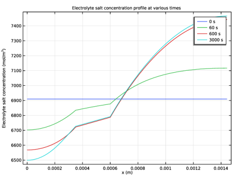
In the Model Builder window, expand the Electrolyte Salt Concentration (batbe) node, then click Line Graph 1.
2
In the Settings window for Line Graph, locate the Legends section.
3
Select the Show legends check box.
4
In the Electrolyte Salt Concentration (batbe) toolbar, click  Plot.
1D Plot Group 7
1
In the Home toolbar, click  Add Plot Group and choose 1D Plot Group.
2
In the Settings window for 1D Plot Group, locate the Data section.
3
From the Time selection list, choose From list.
4
In the Times (s) list, choose 60, 600, and 3000.
5
Locate the Title section. From the Title type list, choose Manual.
6
In the Title text area, type Electrochemical current source at various times.
7
Locate the Plot Settings section.
8
Select the x-axis label check box. In the associated text field, type x (m).
9
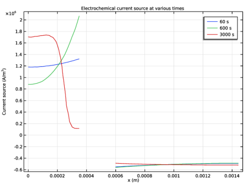
Select the y-axis label check box. In the associated text field, type Current source (A/m<sup>3</sup>).
Line Graph 1
1
Right-click 1D Plot Group 7 and choose Line Graph.
2
In the Settings window for Line Graph, locate the Selection section.
3
From the Selection list, choose All domains.
4
Locate the y-Axis Data section. In the Expression text field, type batbe.iv_per1.
5
Locate the Legends section. Select the Show legends check box.
6
In the 1D Plot Group 7 toolbar, click  Plot.
Current source
1
In the Model Builder window, under Results click 1D Plot Group 7.
2
In the Settings window for 1D Plot Group, type Current source in the Label text field.
1D Plot Group 8
1
In the Home toolbar, click  Add Plot Group and choose 1D Plot Group.
2
In the Settings window for 1D Plot Group, locate the Data section.
3
From the Time selection list, choose From list.
4
In the Times (s) list, choose 60, 600, and 3000.
5
Locate the Title section. From the Title type list, choose Manual.
6
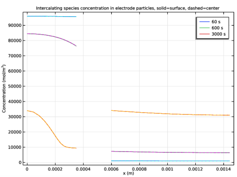
In the Title text area, type Intercalating species concentration in electrode particles, solid=surface, dashed=center.
7
Locate the Plot Settings section.
8
Select the x-axis label check box. In the associated text field, type x (m).
9
Select the y-axis label check box. In the associated text field, type Concentration (mol/m<sup>3</sup>).
Line Graph 1
1
Right-click 1D Plot Group 8 and choose Line Graph.
2
In the Settings window for Line Graph, locate the Selection section.
3
From the Selection list, choose All domains.
4
Click Replace Expression in the upper-right corner of the y-Axis Data section. From the menu, choose Component 1 (comp1)>Battery with Binary Electrolyte>Particle intercalation>batbe.cs_surface - Insertion particle concentration, surface - mol/m³.
5
Locate the Legends section. Select the Show legends check box.
Line Graph 2
1
In the Model Builder window, right-click 1D Plot Group 8 and choose Line Graph.
2
In the Settings window for Line Graph, locate the Selection section.
3
From the Selection list, choose All domains.
4
Click Replace Expression in the upper-right corner of the y-Axis Data section. From the menu, choose Component 1 (comp1)>Battery with Binary Electrolyte>Particle intercalation>batbe.cs_center - Insertion particle concentration, center - mol/m³.
5
Click to expand the Coloring and Style section. Find the Line style subsection. From the Line list, choose Dashed.
6
In the 1D Plot Group 8 toolbar, click  Plot.
Concentration in solid phase
1
In the Model Builder window, under Results click 1D Plot Group 8.
2
In the Settings window for 1D Plot Group, type Concentration in solid phase in the Label text field.