PDF

Liquid-Cooled Lithium-Ion Battery Pack
Introduction
This example simulates a temperature profile in a number of cells and cooling fins in a liquid-cooled battery pack. The model solves in 3D and for an operational point during a load cycle. A full 1D electrochemical model for the lithium battery calculates the average heat source (see also Thermal Modeling of a Cylindrical Lithium-Ion Battery in 3D).
The model is based on two assumptions: The first one is that the material properties of the cooling fluid and battery material can be calculated using an average temperature for the battery pack, and the second one is that the variations in heat generation during the load cycle are significantly slower than the heat transport within the battery pack. The first assumption is valid if the temperature variations in the battery pack are small. The second assumption implies that the thermal balance is quasistationary for the given battery heat source and at a given operational point during the load cycle.
Model Definition
Cell Model
The 1D cell model is identical to the one used in the Thermal Modeling of a Cylindrical Lithium-Ion Battery in 3D model. The battery temperature is set to the inlet temperature of the cooling fluid. The discharge load is set to a 7.5C rate (a full discharge in 1/7.5 of an hour, 480 s).
Flow and Heat Transfer Model
The model uses the Laminar Flow interface to solve for the velocity and pressure in the cooling channels and the Heat Transfer interface for the temperature field.
Geometry
The repetitive unit cell of the battery pack consists of a cooling fin with flow channels, with one battery on each side; see Figure 1. The cooling fins and batteries are 2 mm thick each, summing up to a total unit cell thickness of 6 mm.
Figure 1: Unit cell of the battery pack consisting of two prismatic batteries and a cooling fin plate with five cooling channels.
The modeled battery pack geometry consists of three stacked unit cells and two flow connector channels: one on the inlet and one on the outlet side of the cooling fins (see Figure 2). The geometry represents the last cells toward the outlet end of a battery pack (the cells of the battery pack not included in the geometry extend from y = 0 in the negative y direction).
Figure 2: Battery pack geometry. Three unit cells, one inlet connector channel and one outlet connector channel.
Flow Domain Settings
The flow compartment consists of the two connector channels and the channels in the cooling fins.
The cooling fluid is modeled using the material properties of water. The fluid properties are calculated using the inlet temperature as input.
Flow Boundary Conditions
Since the cells modeled are the last ones in a larger battery pack, and the geometry being modeled is not the complete pack, the flow compartment has two inlets. The flow through the modeled cooling fin plates enters at Inlet 1, whereas the flow that have passed the cooling fins earlier in the battery pack (that are not included in the model) enter at Inlet 2.
An average flow of  = 0.5 cm3/s is assumed for each fin in the battery pack. Defining the number of modeled cooling fins as Nfins, model = 3, and the total number of cooling fins in the pack as Nfins, pack = 50, the inflow conditions are set to
These inflows are set by using the Laminar inflow condition in the Inlet nodes.
At the outlet, atmospheric pressure is applied. All other boundaries are set to no slip conditions.
Heat Transfer Domain Settings
The temperature field is solved for in the flow compartment, the cooling fins, and the batteries.
The cooling fins are made of aluminum. The density, heat capacity, and heat source in the battery domains are set up in the same way as in the Thermal Modeling of a Cylindrical Lithium-Ion Battery in 3D model. The prismatic design of the batteries with the battery sheets primarily extending into the xz-plane results in the following values for the thermal conductivities.
where Li are the thicknesses of the different layers of the cell, and kT,i the thermal conductivities of the materials constituting these layers.
The velocity from the flow model is used as model input for the velocity in the fluid.
Heat Transfer Boundary Conditions
At Inlet 1 an inlet temperature of 310 K for the cooling fluid is specified.
If the flow through each cooling fin is similar, and a similar amount of heat is generated in dissipated from each battery cell in the pack, the fluid temperature at the outlet of each fin will be roughly the same, resulting in a uniform temperature in the outlet cooling channel. For the boundary condition at Inlet 2, a zero temperature gradient in the normal direction is applied (a zero conductive heat flux). This is equal to the default Thermal Insulation condition.
An outflow condition is applied at the outlet and symmetry conditions are applied to the surface of the battery facing the part of the battery pack not included in the geometry (= 0).
On all other boundaries a heat flux conditions is applied with a heat transfer coefficient of 1 W/(m2·K), thus accounting for some heat being lost to the surroundings due to poor insulation.
Solver Sequence
The model is solved sequentially in three studies, one study for each physics interface. The fluid flow is solved for first, using a constant temperature (the inlet temperature), thereby using the assumption of a uniform temperature and the properties of the cooling fluid being constant in the channels.
To calculate the average heat source from the batteries, a second study containing a time-dependent study step is defined solving the 1D battery model only. The simulation is run from the initial conditions of the battery to a desired time, in this case 60 s. The temperature in the battery model is assumed to be constant and equal to the inlet temperature of the cooling fluid.
Finally, the quasi-stationary temperature of the battery pack, at the desired time in the load cycle, is solved for in a stationary study step contained in a third study, using the flow velocity from the first study and the average heat source taken from the last time step of the time-dependent simulation from the second study.
Results and Discussion
Figure 3 shows the pressure in the fluid compartment.
Figure 3: Pressure in the flow compartment.
The velocity magnitude in a cut plane through the middle of one of the cooling fins is shown in Figure 4. The velocity magnitude is about 0.2 m/s in the middle of the channels. This implies that the residence time for the fluid time in the plates is in the range of a only a few seconds, giving support to the assumption that the battery pack reaches a quasi-stationary temperature profile quickly after a load change.
Figure 4: Velocity magnitude in the first cooling fin.
Figure 5 shows the temperature in the batteries. The difference between the highest and lowest temperature in the pack is about 3 K. The temperature variation between different batteries along the y-axis is smaller than the temperature variation within a single battery in the xz-plane.
Figure 5: Temperature in the batteries.
Figure 6 plots the temperature of the cooling fluid. The temperatures are slightly lower than in the battery.
Figure 6: Temperature of the cooling liquid.
Figure 7 shows the temperature in the second battery by comparing the temperature at the surface facing the cooling fin (y = 4 mm) to the surface facing the third battery (y = 6 mm). The surface toward the cooling fin is cooler, reaching a minimum at the corner toward the inlet. The temperature gradient over the battery is also at its maximum at this point.
Figure 7: Temperature increase (in relation to the inlet temperature) of the second battery at the surface facing the cooling fin (y = 4 mm) and the surface facing the third battery (y = 6 mm).
Notes About the COMSOL Implementation
Enable pseudo time stepping for the Laminar Flow interface to improve convergence.
An alternative to approximating the inflow velocity profile is to change the velocity condition to Laminar inflow for the inlet boundary conditions; such an approach requires Vanka smoothing in the Multigrid solver.
Application Library path: Battery_Design_Module/Thermal_Management/li_battery_pack_3d
Modeling Instructions
Application Libraries
1
From the File menu, choose Application Libraries.
2
In the Application Libraries window, select Battery Design Module>Thermal Management>li_battery_1d_for_thermal_models in the tree.
3
Add Component
In the Home toolbar, click  Add Component and choose 3D.
Global Definitions
Replace the parameters from the loaded model with a new set of parameters from a separate file.
Parameters 1
1
In the Model Builder window, under Global Definitions click Parameters 1.
2
In the Settings window for Parameters, locate the Parameters section.
3
Click  Clear Table.
4
In the Model Builder window, click Parameters 1.
5
Click  Load from File.
6
Geometry 2
The model geometry is available as a parameterized geometry sequence in a separate MPH-file. If you want to build it from scratch, follow the instructions in the section Appendix — Geometry Modeling Instructions. Otherwise load it from file with the following steps.
1
In the Geometry toolbar, click Insert Sequence and choose Insert Sequence.
2
3
In the Geometry toolbar, click  Build All.
4
Click  Build All.
5
Click the  Transparency button in the Graphics toolbar.
Turning on transparency makes the channels in the cooling fin visible.
6
Click the  Transparency button in the Graphics toolbar.
Definitions (comp2)
Variables 2
1
In the Home toolbar, click  Variables and choose Local Variables.
2
In the Settings window for Variables, locate the Variables section.
3
Add Physics
1
In the Home toolbar, click  Add Physics to open the Add Physics window.
2
Go to the Add Physics window.
3
In the tree, select Fluid Flow>Single-Phase Flow>Laminar Flow (spf).
4
Click Add to Component 2 in the window toolbar.
5
In the tree, select Heat Transfer>Heat Transfer in Solids and Fluids (ht).
6
Click Add to Component 2 in the window toolbar.
7
In the Home toolbar, click  Add Physics to close the Add Physics window.
Add Study
1
In the Home toolbar, click  Add Study to open the Add Study window.
2
Go to the Add Study window.
3
Find the Studies subsection. In the Select Study tree, select General Studies>Stationary.
4
Click Add Study in the window toolbar.
5
In the Model Builder window, click the root node.
6
In the Home toolbar, click  Add Study to close the Add Study window.
Global Definitions
Step 1 (step1)
In the Home toolbar, click  Functions and choose Global>Step.
Definitions (comp1)
Variables 1
1
In the Settings window for Variables, locate the Variables section.
2
Shared Properties
Model Input 1
1
In the Model Builder window, expand the Component 1 (comp1)>Definitions>Shared Properties node, then click Model Input 1.
2
In the Settings window for Model Input, locate the Definition section.
3
Definitions (comp1)
Average 1 (aveop1)
1
In the Definitions toolbar, click  Nonlocal Couplings and choose Average.
2
In the Settings window for Average, locate the Source Selection section.
3
From the Selection list, choose All domains.
Materials
In the Model Builder window, expand the Component 1 (comp1)>Materials node, then click Component 2 (comp2)>Materials.
Add Material
1
In the Home toolbar, click  Add Material to open the Add Material window.
2
Go to the Add Material window.
3
In the tree, select Built-in>Water, liquid.
4
Click Add to Component in the window toolbar.
5
In the tree, select Built-in>Aluminum.
6
Click Add to Component in the window toolbar.
7
In the Home toolbar, click  Add Material to close the Add Material window.
Materials
Water, liquid (mat4)
1
In the Model Builder window, under Component 2 (comp2)>Materials click Water, liquid (mat4).
2
In the Settings window for Material, locate the Geometric Entity Selection section.
3
From the Selection list, choose Flow compartment.
Aluminum (mat5)
1
In the Model Builder window, click Aluminum (mat5).
2
In the Settings window for Material, locate the Geometric Entity Selection section.
3
From the Selection list, choose Cooling Fins.
Geometry 2
In the Model Builder window, collapse the Component 2 (comp2)>Geometry 2 node.
Materials
Aluminum (mat5)
1
In the Model Builder window, expand the Component 2 (comp2)>Materials>Aluminum (mat5) node, then click Aluminum (mat5).
2
In the Settings window for Material, locate the Material Contents section.
3
4
In the Model Builder window, collapse the Aluminum (mat5) node.
Laminar Flow (spf)
1
In the Model Builder window, under Component 2 (comp2) click Laminar Flow (spf).
2
In the Settings window for Laminar Flow, locate the Domain Selection section.
3
From the Selection list, choose Flow compartment.
Inlet 1
1
In the Physics toolbar, click  Boundaries and choose Inlet.
2
In the Settings window for Inlet, locate the Boundary Selection section.
3
From the Selection list, choose Inlet.
4
Locate the Boundary Condition section. From the list, choose Fully developed flow.
5
Locate the Fully Developed Flow section. Click the Flow rate button.
6
In the V0 text field, type N_fins_model*fin_flow.
Inlet 2
1
In the Physics toolbar, click  Boundaries and choose Inlet.
2
In the Settings window for Inlet, locate the Boundary Selection section.
3
From the Selection list, choose Inlet on outlet flow connector channel.
4
Locate the Boundary Condition section. From the list, choose Fully developed flow.
5
Locate the Fully Developed Flow section. Click the Flow rate button.
6
In the V0 text field, type (N_fins_pack-N_fins_model)*fin_flow.
Outlet 1
1
In the Physics toolbar, click  Boundaries and choose Outlet.
2
In the Settings window for Outlet, locate the Boundary Selection section.
3
From the Selection list, choose Outlet.
4
Locate the Pressure Conditions section. Select the Normal flow check box.
Initial Values 2
1
In the Physics toolbar, click  Domains and choose Initial Values.
2
In the Settings window for Initial Values, locate the Domain Selection section.
3
From the Selection list, choose Block 4 - Outlet flow connector channel.
4
Locate the Initial Values section. Specify the u vector as
Heat Transfer in Solids and Fluids (ht)
Initial Values 1
1
In the Model Builder window, under Component 2 (comp2)>Heat Transfer in Solids and Fluids (ht) click Initial Values 1.
2
In the Settings window for Initial Values, locate the Initial Values section.
3
In the T text field, type T_init.
Fluid 1
1
In the Model Builder window, click Fluid 1.
2
In the Settings window for Fluid, locate the Domain Selection section.
3
From the Selection list, choose Flow compartment.
Battery Layers 1
1
In the Physics toolbar, click  Domains and choose Battery Layers.
2
In the Settings window for Battery Layers, locate the Domain Selection section.
3
From the Selection list, choose Array 1  - Batteries.
4
Click the  Zoom Box button in the Graphics toolbar.
5
In the Model Builder window, click Battery Layers 1.
6
Locate the Battery Layers section. From the Through-layer direction list, choose y-axis.
7
In the ktl text field, type kT_batt_tl.
8
In the kil text field, type kT_batt_il.
9
In the ρeff text field, type rho_batt.
10
In the Cp,eff text field, type Cp_batt.
Heat Source 1
1
In the Physics toolbar, click  Domains and choose Heat Source.
2
In the Settings window for Heat Source, locate the Domain Selection section.
3
From the Selection list, choose Array 2  - Batteries.
4
Locate the Heat Source section. In the Q0 text field, type Qh.
Temperature 1
1
In the Physics toolbar, click  Boundaries and choose Temperature.
2
In the Settings window for Temperature, locate the Boundary Selection section.
3
From the Selection list, choose Inlet.
4
Locate the Temperature section. In the T0 text field, type T_inlet.
Outflow 1
1
In the Physics toolbar, click  Boundaries and choose Outflow.
2
In the Settings window for Outflow, locate the Boundary Selection section.
3
From the Selection list, choose Outlet.
Heat Flux 1
1
In the Physics toolbar, click  Boundaries and choose Heat Flux.
2
In the Settings window for Heat Flux, locate the Boundary Selection section.
3
From the Selection list, choose External heat flux boundaries.
4
Locate the Heat Flux section. From the Flux type list, choose Convective heat flux.
5
In the h text field, type 1.
Symmetry 1
1
In the Physics toolbar, click  Boundaries and choose Symmetry.
2
Multiphysics
Nonisothermal Flow 1 (nitf1)
In the Physics toolbar, click  Multiphysics Couplings and choose Domain>Nonisothermal Flow.
Mesh 2
Size 1
In the Model Builder window, under Component 2 (comp2) right-click Mesh 2 and choose Size.
Size
1
In the Settings window for Size, locate the Element Size section.
2
Click the Custom button.
3
Locate the Element Size Parameters section. In the Maximum element size text field, type 0.009[m].
4
In the Minimum element size text field, type 0.00025[m].
Size 1
1
In the Model Builder window, click Size 1.
2
In the Settings window for Size, locate the Geometric Entity Selection section.
3
From the Geometric entity level list, choose Domain.
4
From the Selection list, choose Flow plate channels.
5
Locate the Element Size section. Click the Custom button.
6
Locate the Element Size Parameters section.
7
Select the Resolution of narrow regions check box. In the associated text field, type 0.2.
Size 2
1
Right-click Component 2 (comp2)>Mesh 2>Size 1 and choose Duplicate.
2
In the Settings window for Size, locate the Geometric Entity Selection section.
3
From the Selection list, choose Block 5 - Inlet flow connector channel.
4
Locate the Element Size Parameters section. In the Resolution of narrow regions text field, type 0.5.
5
Clear the Resolution of narrow regions check box.
6
Select the Maximum element size check box. In the associated text field, type 1.9.
Size 3
1
Right-click Size 2 and choose Duplicate.
2
In the Settings window for Size, locate the Geometric Entity Selection section.
3
From the Selection list, choose Block 4 - Outlet flow connector channel.
Size 4
1
Right-click Size 3 and choose Duplicate.
2
In the Settings window for Size, locate the Geometric Entity Selection section.
3
From the Geometric entity level list, choose Edge.
4
From the Selection list, choose Flow plate channel inlet/outlet edges.
5
Locate the Element Size Parameters section. In the Maximum element size text field, type 0.25.
Free Tetrahedral 1
1
In the Mesh toolbar, click  Free Tetrahedral.
2
In the Settings window for Free Tetrahedral, locate the Domain Selection section.
3
From the Geometric entity level list, choose Domain.
4
From the Selection list, choose Flow compartment.
Boundary Layers 1
1
In the Mesh toolbar, click  Boundary Layers.
2
In the Settings window for Boundary Layers, locate the Geometric Entity Selection section.
3
From the Geometric entity level list, choose Domain.
4
From the Selection list, choose Flow plate channels.
Boundary Layer Properties
1
In the Model Builder window, click Boundary Layer Properties.
2
In the Settings window for Boundary Layer Properties, locate the Boundary Selection section.
3
From the Selection list, choose Flow compartment boundaries.
4
Locate the Layers section. In the Number of layers text field, type 2.
5
From the Thickness specification list, choose First layer.
6
In the Thickness text field, type 0.075.
Free Tetrahedral 2
In the Mesh toolbar, click  Free Tetrahedral.
Size 1
1
Right-click Free Tetrahedral 2 and choose Size.
2
In the Settings window for Size, locate the Element Size section.
3
Click the Custom button.
4
Locate the Element Size Parameters section.
5
Select the Maximum element size check box. In the associated text field, type 6.
6
Click  Build All.
Study 1
Solve the problem using three studies. The first study solves for the flow.
Step 1: Stationary
1
In the Model Builder window, under Study 1 click Step 1: Stationary.
2
In the Settings window for Stationary, locate the Physics and Variables Selection section.
3
In the table, clear the Solve for check boxes for Lithium-Ion Battery (liion) and Heat Transfer in Solids and Fluids (ht).
4
Click to expand the Results While Solving section. From the Probes list, choose None.
The probes from the 1D model are only relevant when the Lithium-Ion Battery interface is active.
5
In the Model Builder window, click Study 1.
6
In the Settings window for Study, locate the Study Settings section.
7
Clear the Generate default plots check box.
8
In the Home toolbar, click  Compute.
Root
Now create a time-dependent study to solve the battery model up to one minute into the load curve.
Add Study
1
In the Home toolbar, click  Add Study to open the Add Study window.
2
Go to the Add Study window.
3
Find the Studies subsection. In the Select Study tree, select General Studies>Time Dependent.
4
Click Add Study in the window toolbar.
Study 2
Step 1: Time Dependent
1
In the Settings window for Time Dependent, locate the Study Settings section.
2
In the Output times text field, type range(0,60,60).
3
Locate the Physics and Variables Selection section. In the table, clear the Solve for check boxes for Laminar Flow (spf) and Heat Transfer in Solids and Fluids (ht).
4
Click to expand the Values of Dependent Variables section. Find the Values of variables not solved for subsection. From the Settings list, choose User controlled.
Use the solution from the first study as initial values to keep the solution for the flow also in this study.
5
From the Method list, choose Solution.
6
From the Study list, choose Study 1, Stationary.
Solution 2 (sol2)
1
In the Study toolbar, click  Show Default Solver.
2
In the Model Builder window, expand the Solution 2 (sol2) node.
3
In the Model Builder window, expand the Study 2>Solver Configurations>Solution 2 (sol2)>Time-Dependent Solver 1 node, then click Fully Coupled 1.
4
In the Settings window for Fully Coupled, click to expand the Method and Termination section.
5
In the Maximum number of iterations text field, type 10.
6
In the Model Builder window, click Study 2.
7
In the Settings window for Study, locate the Study Settings section.
8
Clear the Generate default plots check box.
9
In the Study toolbar, click  Compute.
Root
Finally, create a last study to solve for the temperature profile.
Add Study
1
Go to the Add Study window.
2
Find the Studies subsection. In the Select Study tree, select General Studies>Stationary.
3
Click Add Study in the window toolbar.
4
In the Study toolbar, click  Add Study to close the Add Study window.
Study 3
Step 1: Stationary
1
In the Settings window for Stationary, locate the Results While Solving section.
2
From the Probes list, choose None.
3
Locate the Physics and Variables Selection section. In the table, clear the Solve for check boxes for Lithium-Ion Battery (liion) and Laminar Flow (spf).
4
Click to expand the Values of Dependent Variables section. Find the Values of variables not solved for subsection. From the Settings list, choose User controlled.
5
From the Method list, choose Solution.
6
From the Study list, choose Study 2, Time Dependent.
7
In the Model Builder window, click Study 3.
8
In the Settings window for Study, locate the Study Settings section.
9
Clear the Generate default plots check box.
10
In the Study toolbar, click  Compute.
Results
Study 1/Solution 1 (8) (sol1)
The following steps create a plot of the pressure in the flow compartment (Figure 3).
1
In the Results toolbar, click  More Datasets and choose Solution.
2
In the Settings window for Solution, locate the Solution section.
3
From the Solution list, choose Solution 3 (sol3).
4
From the Component list, choose Component 2 (comp2).
Selection
1
Right-click Study 3/Solution 3 (8) (sol3) and choose Selection.
2
In the Settings window for Selection, locate the Geometric Entity Selection section.
3
From the Geometric entity level list, choose Domain.
4
From the Selection list, choose Flow plate channels.
5
Select the Propagate to lower dimensions check box.
3D Plot Group 2
1
In the Results toolbar, click  3D Plot Group.
2
In the Settings window for 3D Plot Group, locate the Data section.
3
From the Dataset list, choose Study 3/Solution 3 (8) (sol3).
Surface 1
1
Right-click 3D Plot Group 2 and choose Surface.
2
In the Settings window for Surface, locate the Expression section.
3
In the Expression text field, type p.
4
In the 3D Plot Group 2 toolbar, click  Plot.
5
Click the  Zoom Extents button in the Graphics toolbar.
3D Plot Group 3
The following steps create a plot of the temperature in the flow compartment (Figure 6).
1
In the Home toolbar, click  Add Plot Group and choose 3D Plot Group.
2
In the Settings window for 3D Plot Group, locate the Data section.
3
From the Dataset list, choose Study 3/Solution 3 (8) (sol3).
Surface 1
1
Right-click 3D Plot Group 3 and choose Surface.
2
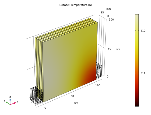
In the Settings window for Surface, click Replace Expression in the upper-right corner of the Expression section. From the menu, choose Component 2 (comp2)>Heat Transfer in Solids and Fluids>Temperature>T - Temperature - K.
3
Locate the Coloring and Style section. Click  Change Color Table.
4
In the Color Table dialog box, select Thermal>ThermalDark in the tree.
5
6
In the 3D Plot Group 3 toolbar, click  Plot.
7
Click the  Zoom Extents button in the Graphics toolbar.
Study 1/Solution 1 (9) (sol1)
The following steps create a surface plot of the velocity magnitude in the first cooling fin (Figure 4).
1
In the Results toolbar, click  More Datasets and choose Solution.
2
In the Settings window for Solution, locate the Solution section.
3
From the Solution list, choose Solution 3 (sol3).
4
From the Component list, choose Component 2 (comp2).
Selection
1
In the Results toolbar, click  Attributes and choose Selection.
2
In the Settings window for Selection, locate the Geometric Entity Selection section.
3
From the Geometric entity level list, choose Domain.
4
From the Selection list, choose Flow plate channels.
Cut Plane 1
1
In the Results toolbar, click  Cut Plane.
2
In the Settings window for Cut Plane, locate the Data section.
3
From the Dataset list, choose Study 3/Solution 3 (9) (sol3).
4
Locate the Plane Data section. From the Plane list, choose xz-planes.
5
In the y-coordinate text field, type 3[mm].
6
2D Plot Group 4
In the Results toolbar, click  2D Plot Group.
Surface 1
1
Right-click 2D Plot Group 4 and choose Surface.
2
In the 2D Plot Group 4 toolbar, click  Plot.
3
Click the  Zoom Extents button in the Graphics toolbar.
Study 1/Solution 1 (10) (sol1)
The following steps create a plot of the temperature on the surface of all battery domains (Figure 5).
1
In the Results toolbar, click  More Datasets and choose Solution.
2
In the Settings window for Solution, locate the Solution section.
3
From the Solution list, choose Solution 3 (sol3).
4
From the Component list, choose Component 2 (comp2).
Selection
1
In the Results toolbar, click  Attributes and choose Selection.
2
In the Settings window for Selection, locate the Geometric Entity Selection section.
3
From the Geometric entity level list, choose Domain.
4
From the Selection list, choose Array 2  - Batteries.
5
Select the Propagate to lower dimensions check box.
3D Plot Group 5
In the Results toolbar, click  3D Plot Group.
Surface 1
1
Right-click 3D Plot Group 5 and choose Surface.
2
In the Settings window for Surface, locate the Data section.
3
From the Dataset list, choose Study 3/Solution 3 (10) (sol3).
4
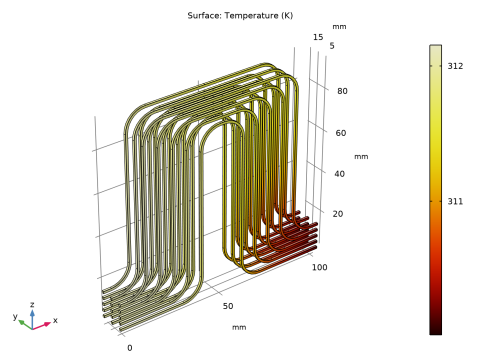
Click Replace Expression in the upper-right corner of the Expression section. From the menu, choose Component 2 (comp2)>Heat Transfer in Solids and Fluids>Temperature>T - Temperature - K.
5
Locate the Coloring and Style section. Click  Change Color Table.
6
In the Color Table dialog box, select Thermal>ThermalDark in the tree.
7
8
In the 3D Plot Group 5 toolbar, click  Plot.
9
Click the  Zoom Extents button in the Graphics toolbar.
Cut Plane 2
The following steps show the temperature increase of the second battery (in relation to the inlet temperature) at the surface facing the cooling fin and the surface facing the third battery (Figure 7).
1
In the Results toolbar, click  Cut Plane.
2
In the Settings window for Cut Plane, locate the Data section.
3
From the Dataset list, choose Study 3/Solution 3 (10) (sol3).
4
Locate the Plane Data section. From the Plane list, choose xz-planes.
5
In the y-coordinate text field, type 4[mm].
2D Plot Group 6
1
In the Results toolbar, click  2D Plot Group.
2
In the Settings window for 2D Plot Group, locate the Data section.
3
From the Dataset list, choose Cut Plane 2.
Surface 1
1
Right-click 2D Plot Group 6 and choose Surface.
2
In the Settings window for Surface, locate the Expression section.
3
In the Expression text field, type T-T_inlet.
4
Click to expand the Range section. Select the Manual color range check box.
5
In the Maximum text field, type 3.
6
Locate the Coloring and Style section. Click  Change Color Table.
7
In the Color Table dialog box, select Thermal>ThermalDark in the tree.
8
Height Expression 1
Right-click Surface 1 and choose Height Expression.
Cut Plane 3
1
In the Results toolbar, click  Cut Plane.
2
In the Settings window for Cut Plane, locate the Data section.
3
From the Dataset list, choose Study 3/Solution 3 (10) (sol3).
4
Locate the Plane Data section. From the Plane list, choose xz-planes.
5
In the y-coordinate text field, type 6[mm].
Surface 2
1
In the Model Builder window, right-click 2D Plot Group 6 and choose Surface.
2
In the Settings window for Surface, locate the Data section.
3
From the Dataset list, choose Cut Plane 3.
4
Locate the Expression section. In the Expression text field, type T-T_inlet.
5
Locate the Range section. Select the Manual color range check box.
6
In the Maximum text field, type 3.
7
Locate the Coloring and Style section. Click  Change Color Table.
8
In the Color Table dialog box, select Thermal>ThermalDark in the tree.
9
10
In the Settings window for Surface, locate the Coloring and Style section.
11
Clear the Color legend check box.
Height Expression 1
1
Right-click Surface 2 and choose Height Expression.
2
In the 2D Plot Group 6 toolbar, click  Plot.
3
Click the  Zoom Extents button in the Graphics toolbar.
Appendix — Geometry Modeling Instructions
From the File menu, choose New.
New
In the New window, click  Blank Model.
Global Definitions
Parameters 1
1
In the Model Builder window, under Global Definitions click Parameters 1.
2
In the Settings window for Parameters, locate the Parameters section.
3
Add Component
In the Home toolbar, click  Add Component and choose 3D.
Geometry 1
1
In the Settings window for Geometry, locate the Units section.
2
From the Length unit list, choose mm.
Block 1 - Batteries
1
In the Geometry toolbar, click  Block.
2
In the Settings window for Block, type Block 1 - Batteries in the Label text field.
3
Locate the Size and Shape section. In the Width text field, type 100.
4
In the Depth text field, type 2.
5
In the Height text field, type 100.
Array 1 - Batteries
1
In the Geometry toolbar, click  Transforms and choose Array.
2
3
In the Settings window for Array, locate the Size section.
4
In the y size text field, type 2.
5
In the Label text field, type Array 1 - Batteries.
6
Locate the Displacement section. In the y text field, type 4.
7
Locate the Selections of Resulting Entities section. Select the Resulting objects selection check box.
Array 2 - Batteries
1
In the Geometry toolbar, click  Transforms and choose Array.
2
In the Settings window for Array, locate the Input section.
3
From the Input objects list, choose Array 1  - Batteries.
4
Locate the Size section. In the y size text field, type N_fins_model.
5
In the Label text field, type Array 2 - Batteries.
6
Locate the Displacement section. In the y text field, type 6.
7
Locate the Selections of Resulting Entities section. Select the Resulting objects selection check box.
Block 2 - Cooling Fins
1
In the Geometry toolbar, click  Block.
2
In the Settings window for Block, type Block 2 - Cooling Fins in the Label text field.
3
Locate the Size and Shape section. In the Width text field, type 100.
4
In the Depth text field, type 2.
5
In the Height text field, type 100.
6
Locate the Position section. In the y text field, type 2.
Block 3 (blk3)
1
In the Geometry toolbar, click  Block.
2
In the Settings window for Block, locate the Size and Shape section.
3
In the Width text field, type 13.
4
In the Depth text field, type 2.
5
In the Height text field, type 20.
6
Locate the Position section. In the x text field, type -13.
7
In the y text field, type 2.
Mirror 1 (mir1)
1
In the Geometry toolbar, click  Transforms and choose Mirror.
2
3
In the Settings window for Mirror, locate the Point on Plane of Reflection section.
4
In the x text field, type 50.
5
Locate the Input section. Select the Keep input objects check box.
6
Locate the Normal Vector to Plane of Reflection section. In the x text field, type 1.
7
In the z text field, type 0.
Union 1 - Cooling Fins
1
In the Geometry toolbar, click  Booleans and Partitions and choose Union.
2
In the Settings window for Union, type Union 1 - Cooling Fins in the Label text field.
3
Locate the Union section. Clear the Keep interior boundaries check box.
4
Locate the Selections of Resulting Entities section. Select the Resulting objects selection check box.
5
Select the objects blk2, blk3, and mir1 only.
Work Plane 1 (wp1)
1
In the Geometry toolbar, click  Work Plane.
2
In the Settings window for Work Plane, locate the Plane Definition section.
3
From the Plane list, choose zx-plane.
4
In the y-coordinate text field, type 2.5.
Work Plane 1 (wp1)>Plane Geometry
In the Model Builder window, click Plane Geometry.
Work Plane 1 (wp1)>Rectangle 1 (r1)
1
In the Work Plane toolbar, click  Rectangle.
2
In the Settings window for Rectangle, locate the Selections of Resulting Entities section.
3
Find the Cumulative selection subsection. Click New.
4
In the New Cumulative Selection dialog box, type Flow plate channels in the Name text field.
5
6
In the Settings window for Rectangle, locate the Size and Shape section.
7
In the Height text field, type 32.
8
Locate the Position section. In the xw text field, type 3.
9
In the yw text field, type -2.
Work Plane 1 (wp1)>Rectangle 2 (r2)
1
In the Work Plane toolbar, click  Rectangle.
2
In the Settings window for Rectangle, locate the Selections of Resulting Entities section.
3
Find the Cumulative selection subsection. From the Contribute to list, choose Flow plate channels.
4
Locate the Size and Shape section. In the Height text field, type 25.
5
Locate the Position section. In the xw text field, type 6.
6
In the yw text field, type -2.
Work Plane 1 (wp1)>Rectangle 3 (r3)
1
In the Work Plane toolbar, click  Rectangle.
2
In the Settings window for Rectangle, locate the Selections of Resulting Entities section.
3
Find the Cumulative selection subsection. From the Contribute to list, choose Flow plate channels.
4
Locate the Size and Shape section. In the Height text field, type 18.
5
Locate the Position section. In the xw text field, type 9.
6
In the yw text field, type -2.
Work Plane 1 (wp1)>Rectangle 4 (r4)
1
In the Work Plane toolbar, click  Rectangle.
2
In the Settings window for Rectangle, locate the Selections of Resulting Entities section.
3
Find the Cumulative selection subsection. From the Contribute to list, choose Flow plate channels.
4
Locate the Size and Shape section. In the Height text field, type 11.
5
Locate the Position section. In the xw text field, type 12.
6
In the yw text field, type -2.
Work Plane 1 (wp1)>Rectangle 5 (r5)
1
In the Work Plane toolbar, click  Rectangle.
2
In the Settings window for Rectangle, locate the Selections of Resulting Entities section.
3
Find the Cumulative selection subsection. From the Contribute to list, choose Flow plate channels.
4
Locate the Size and Shape section. In the Height text field, type 4.
5
Locate the Position section. In the xw text field, type 15.
6
In the yw text field, type -2.
Work Plane 1 (wp1)>Rectangle 6 (r6)
1
In the Work Plane toolbar, click  Rectangle.
2
In the Settings window for Rectangle, locate the Selections of Resulting Entities section.
3
Find the Cumulative selection subsection. From the Contribute to list, choose Flow plate channels.
4
Locate the Size and Shape section. In the Width text field, type 60.
5
Locate the Position section. In the xw text field, type 13.
6
In the yw text field, type 39.
Work Plane 1 (wp1)>Circle 1 (c1)
1
In the Work Plane toolbar, click  Circle.
2
In the Settings window for Circle, locate the Size and Shape section.
3
In the Radius text field, type 10.
4
In the Sector angle text field, type 90.
5
Locate the Position section. In the xw text field, type 13.
6
In the yw text field, type 30.
7
Locate the Rotation Angle section. In the Rotation text field, type 90.
8
Click to expand the Layers section. In the table, enter the following settings:
9
Locate the Object Type section. From the Type list, choose Curve.
10
Locate the Selections of Resulting Entities section. Find the Cumulative selection subsection. From the Contribute to list, choose Flow plate channels.
Work Plane 1 (wp1)>Circle 2 (c2)
1
Right-click Component 1 (comp1)>Geometry 1>Work Plane 1 (wp1)>Plane Geometry>Circle 1 (c1) and choose Duplicate.
2
In the Settings window for Circle, locate the Position section.
3
In the xw text field, type 73.
4
In the yw text field, type 49.
5
Locate the Rotation Angle section. In the Rotation text field, type -90.
6
Click  Build Selected.
Work Plane 1 (wp1)>Delete Entities 1 (del1)
1
In the Work Plane toolbar, click  Delete.
2
In the Settings window for Delete Entities, locate the Entities or Objects to Delete section.
3
From the Geometric entity level list, choose Boundary.
4
On the object c1, select Boundaries 1 and 2 only.
5
On the object c2, select Boundaries 1 and 2 only.
Work Plane 1 (wp1)>Copy 1 (copy1)
1
In the Work Plane toolbar, click  Transforms and choose Copy.
2
Select the objects del1(1), del1(2), and r6 only.
3
In the Settings window for Copy, locate the Displacement section.
4
In the xw text field, type 3,6,9,12.
5
In the yw text field, type -7,-14,-21,-28.
6
Locate the Selections of Resulting Entities section. Find the Cumulative selection subsection. From the Contribute to list, choose Flow plate channels.
Work Plane 1 (wp1)>Rectangle 7 (r7)
1
In the Work Plane toolbar, click  Rectangle.
2
In the Settings window for Rectangle, locate the Position section.
3
In the xw text field, type 82.
4
In the yw text field, type 50.
5
Locate the Selections of Resulting Entities section. Find the Cumulative selection subsection. From the Contribute to list, choose Flow plate channels.
Work Plane 1 (wp1)>Rectangle 8 (r8)
1
In the Work Plane toolbar, click  Rectangle.
2
In the Settings window for Rectangle, locate the Size and Shape section.
3
In the Height text field, type 8.
4
Locate the Position section. In the xw text field, type 85.
5
In the yw text field, type 50.
6
Locate the Selections of Resulting Entities section. Find the Cumulative selection subsection. From the Contribute to list, choose Flow plate channels.
Work Plane 1 (wp1)>Rectangle 9 (r9)
1
In the Work Plane toolbar, click  Rectangle.
2
In the Settings window for Rectangle, locate the Size and Shape section.
3
In the Height text field, type 15.
4
Locate the Position section. In the xw text field, type 88.
5
In the yw text field, type 50.
6
Locate the Selections of Resulting Entities section. Find the Cumulative selection subsection. From the Contribute to list, choose Flow plate channels.
Work Plane 1 (wp1)>Rectangle 10 (r10)
1
In the Work Plane toolbar, click  Rectangle.
2
In the Settings window for Rectangle, locate the Size and Shape section.
3
In the Height text field, type 22.
4
Locate the Position section. In the xw text field, type 91.
5
In the yw text field, type 50.
6
Locate the Selections of Resulting Entities section. Find the Cumulative selection subsection. From the Contribute to list, choose Flow plate channels.
Work Plane 1 (wp1)>Rectangle 11 (r11)
1
In the Work Plane toolbar, click  Rectangle.
2
In the Settings window for Rectangle, locate the Size and Shape section.
3
In the Height text field, type 29.
4
Locate the Position section. In the xw text field, type 94.
5
In the yw text field, type 50.
6
Locate the Selections of Resulting Entities section. Find the Cumulative selection subsection. From the Contribute to list, choose Flow plate channels.
Work Plane 1 (wp1)>Mirror 1 (mir1)
1
In the Work Plane toolbar, click  Transforms and choose Mirror.
2
In the Settings window for Mirror, locate the Input section.
3
From the Input objects list, choose Flow plate channels.
4
Select the Keep input objects check box.
5
Locate the Point on Line of Reflection section. In the yw text field, type 50.
6
Locate the Normal Vector to Line of Reflection section. In the xw text field, type 0.
7
In the yw text field, type 1.
8
Locate the Selections of Resulting Entities section. Find the Cumulative selection subsection. From the Contribute to list, choose Flow plate channels.
Work Plane 1 (wp1)>Union 1 (uni1)
1
In the Work Plane toolbar, click  Booleans and Partitions and choose Union.
2
In the Settings window for Union, locate the Union section.
3
From the Input objects list, choose Flow plate channels.
4
Clear the Keep interior boundaries check box.
Extrude 1 - Flow plate channels
1
In the Model Builder window, under Component 1 (comp1)>Geometry 1 right-click Work Plane 1 (wp1) and choose Extrude.
2
In the Settings window for Extrude, type Extrude 1 - Flow plate channels in the Label text field.
3
Locate the Selections of Resulting Entities section. Select the Resulting objects selection check box.
Array 3 - Cooling Fins
1
In the Geometry toolbar, click  Transforms and choose Array.
2
In the Settings window for Array, type Array 3 - Cooling Fins in the Label text field.
3
4
Locate the Size section. In the y size text field, type N_fins_model.
5
Locate the Displacement section. In the y text field, type 6.
6
Locate the Selections of Resulting Entities section. Select the Resulting objects selection check box.
Array 4 - Flow plate channels
1
In the Geometry toolbar, click  Transforms and choose Array.
2
In the Settings window for Array, locate the Input section.
3
From the Input objects list, choose Extrude 1 - Flow plate channels.
4
In the Label text field, type Array 4 - Flow plate channels.
5
Locate the Size section. In the y size text field, type N_fins_model.
6
Locate the Displacement section. In the y text field, type 6.
7
Locate the Selections of Resulting Entities section. Select the Resulting objects selection check box.
Block 4 - Outlet flow connector channel
1
In the Geometry toolbar, click  Block.
2
In the Settings window for Block, locate the Selections of Resulting Entities section.
3
Select the Resulting objects selection check box.
4
In the Label text field, type Block 4 - Outlet flow connector channel.
5
Locate the Size and Shape section. In the Width text field, type 8.
6
In the Depth text field, type 18.
7
In the Height text field, type 16.
8
Locate the Position section. In the x text field, type -10.
9
In the z text field, type 2.
Block 5 - Inlet flow connector channel
1
In the Geometry toolbar, click  Block.
2
In the Settings window for Block, locate the Selections of Resulting Entities section.
3
Select the Resulting objects selection check box.
4
In the Label text field, type Block 5 - Inlet flow connector channel.
5
Locate the Size and Shape section. In the Width text field, type 8.
6
In the Depth text field, type 16.
7
In the Height text field, type 16.
8
Locate the Position section. In the x text field, type 102.
9
In the z text field, type 2.
Difference 1 (dif1)
1
In the Geometry toolbar, click  Booleans and Partitions and choose Difference.
2
In the Settings window for Difference, locate the Difference section.
3
From the Objects to add list, choose Array 3 - Cooling Fins.
4
Find the Objects to subtract subsection. Click to select the  Activate Selection toggle button.
5
Select the objects blk4 and blk5 only.
6
Select the Keep objects to subtract check box.
7
Click  Build Selected.
Form Union (fin)
1
In the Model Builder window, click Form Union (fin).
2
In the Settings window for Form Union/Assembly, click  Build Selected.
3
Click the  Wireframe Rendering button in the Graphics toolbar.
Cooling Fins
1
In the Geometry toolbar, click  Selections and choose Difference Selection.
2
In the Settings window for Difference Selection, type Cooling Fins in the Label text field.
3
Locate the Input Entities section. Click  Add.
4
In the Add dialog box, select Array 3 - Cooling Fins in the Selections to add list.
5
6
In the Settings window for Difference Selection, locate the Input Entities section.
7
8
In the Add dialog box, select Array 4 - Flow plate channels in the Selections to subtract list.
9
Flow compartment
1
In the Geometry toolbar, click  Selections and choose Union Selection.
2
In the Settings window for Union Selection, type Flow compartment in the Label text field.
3
Locate the Input Entities section. Click  Add.
4
In the Add dialog box, in the Selections to add list, choose Array 4 - Flow plate channels, Block 4 - Outlet flow connector channel, and Block 5 - Inlet flow connector channel.
5
Flow compartment boundaries
1
In the Geometry toolbar, click  Selections and choose Adjacent Selection.
2
In the Settings window for Adjacent Selection, type Flow compartment boundaries in the Label text field.
3
Locate the Input Entities section. Click  Add.
4
In the Add dialog box, select Flow compartment in the Input selections list.
5
Inlet
1
In the Geometry toolbar, click  Selections and choose Explicit Selection.
2
In the Settings window for Explicit Selection, type Inlet in the Label text field.
3
Locate the Entities to Select section. From the Geometric entity level list, choose Boundary.
4
On the object fin, select Boundary 450 only.
Outlet
1
In the Geometry toolbar, click  Selections and choose Explicit Selection.
2
In the Settings window for Explicit Selection, type Outlet in the Label text field.
3
Locate the Entities to Select section. From the Geometric entity level list, choose Boundary.
4
On the object fin, select Boundary 38 only.
Inlet on outlet flow connector channel
1
In the Geometry toolbar, click  Selections and choose Explicit Selection.
2
In the Settings window for Explicit Selection, type Inlet on outlet flow connector channel in the Label text field.
3
Locate the Entities to Select section. From the Geometric entity level list, choose Boundary.
4
On the object fin, select Boundary 17 only.
Boundary toward battery pack
1
In the Geometry toolbar, click  Selections and choose Explicit Selection.
2
In the Settings window for Explicit Selection, type Boundary toward battery pack in the Label text field.
3
Locate the Entities to Select section. From the Geometric entity level list, choose Boundary.
4
On the object fin, select Boundary 122 only.
Geometry
1
In the Geometry toolbar, click  Selections and choose Explicit Selection.
2
In the Settings window for Explicit Selection, type Geometry in the Label text field.
3
Locate the Entities to Select section. From the Geometric entity level list, choose Object.
4
All external boundaries
1
In the Geometry toolbar, click  Selections and choose Adjacent Selection.
2
In the Settings window for Adjacent Selection, type All external boundaries in the Label text field.
3
Locate the Input Entities section. Click  Add.
4
In the Add dialog box, select Geometry in the Input selections list.
5
Difference Selection 2 (difsel2)
In the Geometry toolbar, click  Selections and choose Difference Selection.
Difference Selection 3 (difsel3)
In the Geometry toolbar, click  Selections and choose Difference Selection.
External heat flux boundaries
1
In the Model Builder window, under Component 1 (comp1)>Geometry 1 click Difference Selection 2 (difsel2).
2
In the Settings window for Difference Selection, type External heat flux boundaries in the Label text field.
3
Locate the Geometric Entity Level section. From the Level list, choose Boundary.
4
Locate the Input Entities section. Click  Add.
5
In the Add dialog box, select All external boundaries in the Selections to add list.
6
7
In the Settings window for Difference Selection, locate the Input Entities section.
8
9
In the Add dialog box, in the Selections to subtract list, choose Inlet, Outlet, Inlet on outlet flow connector channel, and Boundary toward battery pack.
10
11
In the Geometry toolbar, click  Build All.
Flow plate channels
1
In the Model Builder window, under Component 1 (comp1)>Geometry 1 click Difference Selection 3 (difsel3).
2
In the Settings window for Difference Selection, type Flow plate channels in the Label text field.
3
Locate the Input Entities section. Click  Add.
4
In the Add dialog box, select Flow compartment in the Selections to add list.
5
6
In the Settings window for Difference Selection, locate the Input Entities section.
7
8
In the Add dialog box, in the Selections to subtract list, choose Block 4 - Outlet flow connector channel and Block 5 - Inlet flow connector channel.
9
Flow plate channel boundaries
1
In the Geometry toolbar, click  Selections and choose Adjacent Selection.
2
In the Settings window for Adjacent Selection, type Flow plate channel boundaries in the Label text field.
3
Locate the Input Entities section. Click  Add.
4
In the Add dialog box, select Flow plate channels in the Input selections list.
5
Flow connector channel boundaries
1
In the Geometry toolbar, click  Selections and choose Adjacent Selection.
2
In the Settings window for Adjacent Selection, type Flow connector channel boundaries in the Label text field.
3
Locate the Input Entities section. Click  Add.
4
In the Add dialog box, in the Input selections list, choose Block 4 - Outlet flow connector channel and Block 5 - Inlet flow connector channel.
5
Flow plate channel inlet/outlet boundaries
1
In the Geometry toolbar, click  Selections and choose Intersection Selection.
2
In the Settings window for Intersection Selection, type Flow plate channel inlet/outlet boundaries in the Label text field.
3
Locate the Geometric Entity Level section. From the Level list, choose Boundary.
4
Locate the Input Entities section. Click  Add.
5
In the Add dialog box, in the Selections to intersect list, choose Flow plate channel boundaries and Flow connector channel boundaries.
6
Flow plate channel inlet/outlet edges
1
In the Geometry toolbar, click  Selections and choose Adjacent Selection.
2
In the Settings window for Adjacent Selection, type Flow plate channel inlet/outlet edges in the Label text field.
3
Locate the Input Entities section. From the Geometric entity level list, choose Boundary.
4
5
In the Add dialog box, select Flow plate channel inlet/outlet boundaries in the Input selections list.
6
7
In the Settings window for Adjacent Selection, locate the Output Entities section.
8
From the Geometric entity level list, choose Adjacent edges.
Boundaries for boundary layer mesh
1
In the Geometry toolbar, click  Selections and choose Difference Selection.
2
In the Settings window for Difference Selection, type Boundaries for boundary layer mesh in the Label text field.
3
Locate the Geometric Entity Level section. From the Level list, choose Boundary.
4
Locate the Input Entities section. Click  Add.
5
In the Add dialog box, select Flow compartment boundaries in the Selections to add list.
6
7
In the Settings window for Difference Selection, locate the Input Entities section.
8
9
In the Add dialog box, in the Selections to subtract list, choose Inlet, Outlet, and Inlet on outlet flow connector channel.
10