|
|
|

|
1
|
|
2
|
In the Select Physics tree, select Electrochemistry>Tertiary Current Distribution, Nernst-Planck>Tertiary, Electroneutrality (tcd).
|
|
3
|
Click Add.
|
|
4
|
Click
|
|
5
|
|
6
|
Click
|
|
1
|
|
2
|
|
3
|
|
4
|
Browse to the model’s Application Libraries folder and double-click the file electrochemical_capacitor_porous_electrodes_cell_parameters.txt.
|
|
5
|
|
1
|
|
2
|
|
3
|
|
4
|
Browse to the model’s Application Libraries folder and double-click the file electrochemical_capacitor_porous_electrodes_load_parameters.txt.
|
|
1
|
|
2
|
|
3
|
|
4
|
|
6
|
|
1
|
In the Model Builder window, under Component 1 (comp1)>Tertiary Current Distribution, Nernst-Planck (tcd) click Species Charges 1.
|
|
2
|
|
3
|
|
4
|
|
1
|
|
2
|
|
3
|
|
4
|
|
1
|
|
2
|
|
3
|
|
4
|
|
1
|
|
3
|
|
4
|
|
5
|
|
6
|
Locate the Electrode Current Conduction section. From the σs list, choose User defined. In the associated text field, type sigma_s.
|
|
7
|
|
8
|
|
9
|
Locate the Effective Transport Parameter Correction section. From the Diffusion list, choose Tortuosity.
|
|
10
|
|
11
|
Locate the Effective Transport Parameter Correction section. From the Electrical conductivity list, choose Tortuosity.
|
|
12
|
|
13
|
|
15
|
|
16
|
|
1
|
|
2
|
In the Settings window for Porous Matrix Double Layer Capacitance, locate the Porous Matrix Double Layer Capacitance section.
|
|
3
|
|
4
|
|
5
|
|
1
|
|
2
|
|
3
|
In the Reaction rate for dissolving-depositing species table, enter the following settings:
|
|
1
|
|
3
|
|
4
|
|
5
|
|
6
|
|
7
|
Locate the Effective Transport Parameter Correction section. From the Diffusion list, choose Tortuosity.
|
|
8
|
|
1
|
|
2
|
Right-click Tertiary Current Distribution, Nernst-Planck (tcd) and choose Electrode>Electric Ground.
|
|
1
|
|
3
|
|
4
|
|
1
|
|
2
|
|
3
|
|
5
|
|
1
|
|
2
|
|
3
|
|
4
|
|
5
|
|
1
|
|
2
|
|
1
|
|
2
|
|
3
|
|
1
|
|
2
|
|
3
|
|
4
|
|
1
|
|
2
|
|
3
|
|
4
|
|
5
|
|
1
|
|
2
|
|
3
|
|
4
|
|
5
|
|
6
|
Locate the Reinitialization section. In the table, enter the following settings:
|
|
1
|
|
2
|
|
3
|
|
4
|
Click OK.
|
|
5
|
In the Model Builder window, under Component 1 (comp1) click Tertiary Current Distribution, Nernst-Planck (tcd).
|
|
1
|
|
2
|
|
4
|
|
5
|
In the Dependent variable quantity table, enter the following settings:
|
|
1
|
In the Model Builder window, under Component 1 (comp1)>Tertiary Current Distribution, Nernst-Planck (tcd), Ctrl-click to select Electrode Current Density 1 and Global Equations 1.
|
|
2
|
Right-click and choose Group.
|
|
1
|
|
2
|
|
3
|
|
1
|
|
2
|
|
3
|
|
4
|
|
5
|
|
6
|
|
1
|
|
2
|
|
3
|
|
1
|
|
2
|
|
3
|
|
4
|
|
1
|
|
2
|
|
3
|
In the Model Builder window, expand the Study 1: CC Charge CV Discharge>Solver Configurations>Solution 1 (sol1)>Dependent Variables 1 node, then click State variable i_app_ch (comp1.ODE1).
|
|
4
|
|
5
|
|
6
|
|
7
|
In the Model Builder window, under Study 1: CC Charge CV Discharge>Solver Configurations>Solution 1 (sol1) click Time-Dependent Solver 1.
|
|
8
|
|
9
|
|
10
|
|
11
|
|
12
|
|
13
|
Click to expand the Results While Solving section. Right-click Study 1: CC Charge CV Discharge>Solver Configurations>Solution 1 (sol1)>Time-Dependent Solver 1 and choose Stop Condition.
|
|
14
|
|
15
|
Click
|
|
17
|
|
18
|
|
19
|
|
1
|
|
2
|
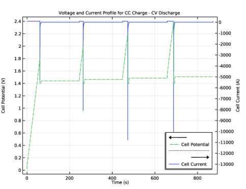
In the Settings window for 1D Plot Group, type Voltage and Current Profile for CC Charge - CV Discharge in the Label text field.
|
|
1
|
|
2
|
|
3
|
|
4
|
|
5
|
|
1
|
In the Model Builder window, right-click Voltage and Current Profile for CC Charge - CV Discharge and choose Point Graph.
|
|
2
|
|
4
|
|
5
|
|
6
|
|
7
|
Click to expand the Coloring and Style section. Find the Line style subsection. From the Line list, choose Dash-dot.
|
|
8
|
|
9
|
|
10
|
Select the Description check box.
|
|
1
|
|
2
|
|
3
|
|
4
|
|
5
|
|
6
|
|
7
|
|
8
|
|
1
|
|
2
|
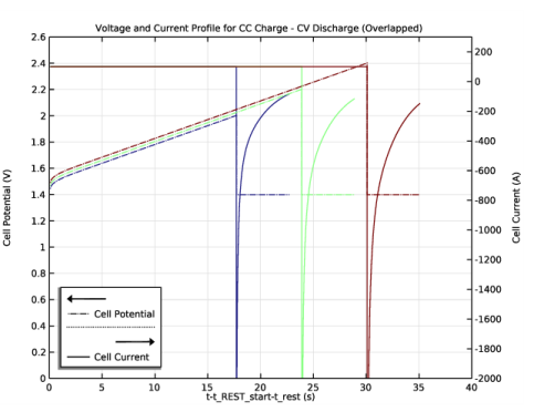
In the Settings window for 1D Plot Group, type Voltage and Current Profile for CC Charge - CV Discharge (Overlapped) in the Label text field.
|
|
1
|
In the Model Builder window, expand the Voltage and Current Profile for CC Charge - CV Discharge (Overlapped) node, then click Current.
|
|
2
|
|
3
|
|
4
|
|
1
|
|
2
|
|
3
|
|
4
|
|
1
|
|
2
|
|
3
|
|
4
|
|
1
|
In the Model Builder window, under Results>Voltage and Current Profile for CC Charge - CV Discharge (Overlapped) click Potential.
|
|
2
|
|
3
|
|
4
|
|
1
|
|
2
|
|
3
|
|
4
|
|
1
|
|
2
|
|
3
|
|
4
|
|
1
|
In the Model Builder window, under Results click Voltage and Current Profile for CC Charge - CV Discharge (Overlapped).
|
|
2
|
|
3
|
|
4
|
|
5
|
|
6
|
|
7
|
|
8
|
|
9
|
|
10
|
|
11
|
|
1
|
|
3
|
|
4
|
|
5
|
|
6
|
|
1
|
|
3
|
|
4
|
|
5
|
|
6
|
|
1
|
In the Model Builder window, under Component 1 (comp1)>Tertiary Current Distribution, Nernst-Planck (tcd), Ctrl-click to select Electrode Power 1 and Initial Values - Constant Power.
|
|
2
|
Right-click and choose Group.
|
|
1
|
|
1
|
|
2
|
|
3
|
|
4
|
|
5
|
|
1
|
|
2
|
|
3
|
In the tree, select Component 1 (comp1)>Tertiary Current Distribution, Nernst-Planck (tcd)>Constant Current Charge/Constant Voltage Discharge.
|
|
4
|
Right-click and choose Disable.
|
|
5
|
|
6
|
|
7
|
|
1
|
|
2
|
|
4
|
|
5
|
Click
|
|
7
|
|
8
|
|
9
|
|
1
|
In the Model Builder window, expand the Study 2: Constant Power Charge>Solver Configurations>Solution 2 (sol2) node, then click Time-Dependent Solver 1.
|
|
2
|
|
3
|
|
1
|
|
2
|
|
3
|
|
1
|
|
3
|
|
4
|
|
5
|
|
6
|
|
7
|
|
8
|
|
9
|
|
10
|
|
11
|
|
12
|
|
1
|
|
2
|
|
3
|
|
4
|
|
5
|
|
1
|
|
2
|
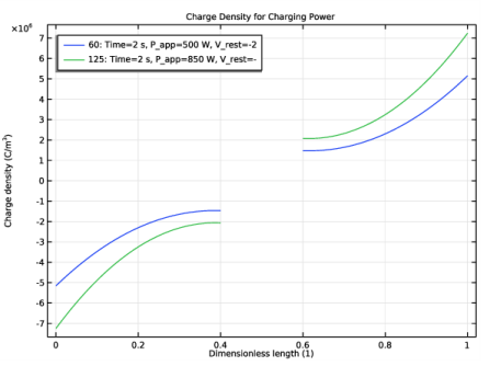
In the Settings window for 1D Plot Group, type Charge Density for Charging Power in the Label text field.
|
|
3
|
Locate the Data section. From the Dataset list, choose Study 2: Constant Power Charge/Solution 2 (sol2).
|
|
4
|
|
5
|
|
1
|
|
2
|
|
3
|
|
4
|
|
5
|
|
6
|
|
7
|
|
8
|
|
1
|
|
2
|
|
3
|
|
4
|
|
5
|
|
6
|
|
1
|
|
2
|
In the Settings window for 1D Plot Group, type Voltage and Current Profiles for Constant Power Charge in the Label text field.
|
|
3
|
Locate the Data section. From the Dataset list, choose Study 2: Constant Power Charge/Solution 2 (sol2).
|
|
4
|
|
1
|
|
2
|
|
4
|
|
5
|
|
6
|
|
7
|
|
8
|
|
9
|
|
1
|
In the Model Builder window, right-click Voltage and Current Profiles for Constant Power Charge and choose Global.
|
|
2
|
|
3
|
Click Replace Expression in the upper-right corner of the y-Axis Data section. From the menu, choose Component 1 (comp1)>Tertiary Current Distribution, Nernst-Planck>tcd.phis0_epow1 - Electric potential on boundary - V.
|
|
4
|
Click to expand the Coloring and Style section. Find the Line style subsection. From the Line list, choose Dash-dot.
|
|
5
|
|
6
|
|
7
|
|
8
|
|
1
|
|
2
|
|
3
|
|
4
|
|
5
|
Select the Secondary y-axis label check box. In the associated text field, type Electric Potential (V).
|
|
6
|
|
7
|
|
8
|
|
9
|
|
10
|
|
11
|
|
12
|
|
13
|
|
14
|
|
15
|
|
16
|