PDF

Open Pipe
Introduction
In this tutorial model, a vibrating piston is mounted inside one end of a cylindrical pipe, while the other end of the pipe opens into an infinite domain. The problem is solved using two different approaches to illustrate their strengths and weaknesses. In the first case, an impedance boundary condition modeling radiation losses into an infinite domain is specified on the pipe end while the acoustics in the domain is not solved explicitly. This is consequently a fast approach. In the second case, a perfectly matched layer condition is applied on the domain. This condition offers a consistent and physically sound method for modeling infinite domains using finite-sized regions. Thus, the domain acoustics is explicitly solved for, but only in a region close to the pipe outlet.
The model considers two different types of pipes: a flanged and an unflanged. In both cases, the impedance-based model is compared with the model using the perfectly matched layer condition.
Model Definition
Figure 1: Sketch of the two pipe geometries considered in this model: the flanged pipe (left) and the unflanged pipe (right).
We consider the acoustics of an open pipe with a harmonically oscillating piston mounted in one end. Figure 1 shows the geometry for the two cases considered: the flanged pipe (left) and an unflanged pipe (right). In both cases, the pipe opens into an unbounded domain, and the piston is mounted at the bottom end of the pipe.
The pipe has length L = 1.5 m and radius a = 0.25 m. The piston provides a harmonically oscillating acceleration an(t) = a0eiωt in the axial direction at the end of the pipe, where ω = 2πf [rad/s] is the angular frequency corresponding to the frequency f [Hz]. The model sweeps in the frequency f, from 10 Hz to 1000 Hz. The acoustic medium is air with the density 1.25 kg m3 and the speed of sound c = 343 m/s.
The axial symmetry of both the physics and the geometry allows us to exploit the 2D axisymmetry interface.
Modeling the unbounded domain
For either geometry, you can model the infinite domain in two separate ways. In the first case, you apply an impedance boundary condition on the pipe outlet, and otherwise ignore the external domain. The impedance is an analytical, geometry-specific model, so the choice of impedance model specifies the geometry of the domain (that is, whether the pipe is flanged or not). This is a computationally efficient method, because you do not need to explicitly model the external domain. However, the analytical expression for the impedance assumes that the incident waves is strictly plane on the outlet. This is always true for low frequencies, but for higher frequencies the geometry can also support nonplane waves. Moreover, the far field of the sound radiation will in this case start to exhibit directivity (a far-field beam pattern with lobes), which will introduce additional deviations for the simple impedance approach. The cutoff frequency is given by Ref. 1
where α = 3.832 is the first root of the Bessel function of the first kind of order 1 and the rest of the parameters are given above. The exact value is fc = 836.76 Hz. Above this frequency, you cannot expect the impedance-based model to provide the exact result.
In the second case, you explicitly model the surrounding domain. To do so, use a perfectly matched layer (PML) condition to model the unboundedness of the domain and therefore only model a finite region. The PML condition is an artificial absorbing layer, which can be used to truncate the domain while still simulating open boundaries. Compared to the impedance-based model, this approach is more computationally heavy because it also solves for the acoustics in the domain, albeit a truncated one. However, because the domain is modeled explicitly, this approach automatically supports frequencies above the cutoff frequency fc where nonplane waves can exist.
Governing equation
Being a time-harmonic problem, this model uses the frequency-domain Helmholtz equation for the sound pressure amplitude p
(1)
where ρ is the density of the air. The full pressure is given by p(t) = peiωt. Comparing to the equation display in the COMSOL Desktop window, Equation 1 does not contain the dipole source q, because no such dipole sources are present in the domain.
Boundary conditions
As already touched upon, you can use two different types of boundary conditions to model the unbounded domain in this problem: an impedance condition imposed on the pipe outlet, or an explicit model of the surrounding domain with a perfectly matched layer to simulate the open boundaries. The former case requires the addition of a separate equation on the boundary as detailed below, while the latter does not.
An impedance boundary condition stipulates a relationship between the pressure p and the boundary-normal velocity v at the pipe outlet. It is defined as Zi = p/v and is typically frequency dependent. The impedance boundary conditions are invoked by imposing the following equation on the open end of the pipe
,
where n is the outward pointing normal vector to the boundary. A complex value of the impedance indicates losses and associated phase-shift between the pressure and the boundary-normal velocity.
In addition to handling the unbounded domain, the model also includes conditions to model the oscillating piston as well as the hard side walls of the pipe and the flange (the latter where applicable). The oscillating piston is modeled by imposing a harmonically oscillating acceleration at the pipe inlet
,
where a0 is the amplitude of the harmonically oscillating acceleration.
For the flanged pipe, the hard walls of the pipe and flange are given by applying the following equation on the appropriate boundaries
(2).
The unflanged pipe furthermore has places with air on both sides of the pipe wall. On these wall segments, the condition above applies to the fluid on both sides,
with the fluid on the two sides of the pipe wall denoted by subscripts ‘1’ and ‘2’, respectively. Wall segments with air on only one side are modeled using Equation 2.
Results and Discussion
Figure 2: Impedance Zi as a function of driving frequency f for the flanged pipe. For the PML model, the implied impedance is derived according to Equation 3.
Flanged pipe
First consider the results from the flanged pipe. We are ultimately interested in comparing the pipe outlet pressure between the two modeling approaches (impedance or PMLs), but an important factor in this regard is to investigate the radiated losses at the pipe outlet. For the impedance-based model, these are exactly what the impedance Zi expresses. To compare this to the model with PMLs, compute an implied impedance on the pipe outlet by taking the ratio of the boundary-average pressure to the boundary-average of the boundary-normal velocity . Thus, since the pipe outlet boundary is circular with radius a, the implied impedance for the PML model is
(3).
Figure 2 shows the result of this comparison. As expected, there is good comparison between the two modeling approaches until the cutoff frequency of fc = 836.76 Hz. Above this, the nonplane waves supported by the geometry are observed to become increasingly influential as the impedance-based model (solid lines) begin to deviate.
Several impedance models have been derived as analytical approximations valid only for limited regimes of the relative wave number k·a. To illustrate this, Figure 3 repeats the plot in Figure 2 but shown as a function of k·a rather than f.
Figure 3: Impedance Zi as a function of relative wave number k·a for the flanged pipe. For the PML model, the implied impedance is derived according to Equation 3.
Finally, compare in Figure 4 the pressure at the centerline of the pipe outlet from the two models. There is good agreement across all frequencies even though the impedances exhibit some variations at higher frequencies (see Figure 2).
Figure 4: Pipe outlet pressure p for the flanged pipe for both impedance and PML models. In spite of noticeable variations for the impedances at higher frequencies (Figure 2), the predicted pressure from the two models is in general in good agreement across all frequencies.
Unflanged pipe
Then repeat the analysis for an unflanged pipe. In this case, the impedance model is an approximate analytical solution valid only for small values of k·a. Figure 5Figure 7 show the results of this analysis; these are analogous to the pipe results above for the flanged pipe and therefore warrant only short mention.
Figure 5 illustrates that the analytical and implied impedances are comparable across the entire frequency range. However, for k·a greater than about 2, the analytical impedance deviates quite significantly; see Figure 6. This is not quite as expected since the impedance model should apply for k·a < 3.83; however, this could be due to the model itself being an approximation, not an exact analytical result even for low k·a. Nonetheless, Figure 7 illustrates that the predicted centerline outlet pressure from either the impedance-based model or the PML model are in fair agreement across the entire range of probed frequencies.
Figure 5: Impedance Zi as a function of driving frequency f for the unflanged pipe. For the PML model, the implied impedance is derived according to Equation 3.
Figure 6: Impedance Zi as a function of driving relative wave number k·a for the unflanged pipe. For the PML model, the implied impedance is derived according to Equation 3.
Figure 7: Pressure p at the centerline of the pipe outlet for the unflanged pipe.
Notes About the COMSOL Implementation
In anticipation of using a frequency sweep covering several decades, define the frequency limits fmin and fmax as exponents without units and set the frequency range to .
Reference
1. D.T. Blackstock, Fundamentals of physical acoustics, John Wiley & Sons, 2000.
Application Library path: Acoustics_Module/Verification_Examples/open_pipe
Modeling Instructions
You start by modeling a flanged pipe. You will be comparing the two different approaches for solving the problem, so start by immediately adding the physics option twice.
From the File menu, choose New.
New
In the New window, click  Model Wizard.
Model Wizard
1
In the Model Wizard window, click  2D Axisymmetric.
2
In the Select Physics tree, select Acoustics>Pressure Acoustics>Pressure Acoustics, Frequency Domain (acpr).
3
Click Add.
4
Click Add.
5
Global Definitions
Parameters 1
1
In the Model Builder window, under Global Definitions click Parameters 1.
2
In the Settings window for Parameters, locate the Parameters section.
3
Click  Load from File.
4
Geometry 1
First model the pipe.
Rectangle 1 (r1)
1
In the Geometry toolbar, click  Rectangle.
2
In the Settings window for Rectangle, locate the Size and Shape section.
3
In the Width text field, type a.
4
In the Height text field, type L.
5
Locate the Position section. In the z text field, type -L.
Now model the surroundings. Only use a quarter circle to model the flange on the pipe.
Circle 1 (c1)
1
In the Geometry toolbar, click  Circle.
2
In the Settings window for Circle, locate the Size and Shape section.
3
In the Radius text field, type 6*a.
4
In the Sector angle text field, type 90.
Add an external layer to the circle. You will later apply the Perfectly Matched Layer (PML) condition in this layer.
5
Click to expand the Layers section. In the table, enter the following settings:
6
Click  Build All Objects.
7
Click the  Zoom Extents button in the Graphics toolbar.
In pressure acoustics you only need to specify the density and speed of sound. When these parameters are known, this is most easily done by adding a blank material and providing the parameter values. Otherwise, add a built-in material. In this case you add the parameter values for air.
Materials
Material 1 (mat1)
1
In the Model Builder window, under Component 1 (comp1) right-click Materials and choose Blank Material.
2
In the Settings window for Material, locate the Material Contents section.
3
Component 1 - Flanged pipe radiation
1
In the Model Builder window, click Component 1 (comp1).
2
In the Settings window for Component, type Component 1 - Flanged pipe radiation in the Label text field.
Set up the model of the flanged pipe using an impedance boundary condition.
Pressure Acoustics, Frequency Domain - impedance model
1
In the Model Builder window, under Component 1 - Flanged pipe radiation (comp1) click Pressure Acoustics, Frequency Domain (acpr).
2
In the Settings window for Pressure Acoustics, Frequency Domain, type Pressure Acoustics, Frequency Domain - impedance model in the Label text field.
3
Normal Acceleration 1
1
In the Physics toolbar, click  Boundaries and choose Normal Acceleration.
2
3
In the Settings window for Normal Acceleration, locate the Normal Acceleration section.
4
In the an text field, type a0.
Impedance 1
1
In the Physics toolbar, click  Boundaries and choose Impedance.
2
3
In the Settings window for Impedance, locate the Impedance section.
4
From the Impedance model list, choose Waveguide end impedance.
5
In the a text field, type a.
Now set up the model of the flanged pipe using a perfectly matched layer condition.
Pressure Acoustics, Frequency Domain 2 - perfectly matched layers
1
In the Model Builder window, under Component 1 - Flanged pipe radiation (comp1) click Pressure Acoustics, Frequency Domain 2 (acpr2).
2
In the Settings window for Pressure Acoustics, Frequency Domain, type Pressure Acoustics, Frequency Domain 2 - perfectly matched layers in the Label text field.
Set up the perfectly matched layer. Also set up a nonlocal integration coupling on the pipe outlet; this operator will be used for postprocessing.
Definitions
Perfectly Matched Layer 1 (pml1)
1
In the Definitions toolbar, click  Perfectly Matched Layer.
2
3
In the Settings window for Perfectly Matched Layer, locate the Scaling section.
4
From the Coordinate stretching type list, choose Rational.
5
From the Physics list, choose Pressure Acoustics, Frequency Domain 2 - perfectly matched layers (acpr2).
6
In the PML scaling factor text field, type 0.5.
7
In the PML scaling curvature parameter text field, type 5.
Definitions
Integration 1 (intop1)
1
In the Definitions toolbar, click  Nonlocal Couplings and choose Integration.
2
In the Settings window for Integration, locate the Source Selection section.
3
From the Geometric entity level list, choose Boundary.
4
Pressure Acoustics, Frequency Domain 2 - perfectly matched layers (acpr2)
Normal Acceleration 1
1
In the Physics toolbar, click  Boundaries and choose Normal Acceleration.
2
3
In the Settings window for Normal Acceleration, locate the Normal Acceleration section.
4
In the an text field, type a0.
Mesh 1
In this model, the mesh is set up manually. Proceed by directly adding the desired mesh component. In general, 5 to 6 second-order elements per wavelength are needed to resolve the waves. For more details, see Meshing (Resolving the Waves) in the Acoustics Module User’s Guide. Here, we use 6 elements per wavelength.
Free Triangular 1
In the Mesh toolbar, click  Free Triangular.
Size
1
In the Model Builder window, click Size.
2
In the Settings window for Size, locate the Element Size section.
3
Click the Custom button.
4
Locate the Element Size Parameters section. In the Maximum element size text field, type hmax.
5
In the Minimum element size text field, type 6.0E-4.
Free Triangular 1
1
In the Model Builder window, click Free Triangular 1.
2
In the Settings window for Free Triangular, locate the Domain Selection section.
3
From the Geometric entity level list, choose Domain.
4
Size 1
1
Right-click Free Triangular 1 and choose Size.
2
In the Settings window for Size, locate the Geometric Entity Selection section.
3
From the Geometric entity level list, choose Point.
4
5
Locate the Element Size section. Click the Custom button.
6
Locate the Element Size Parameters section.
7
Select the Maximum element size check box. In the associated text field, type hmax/15.
Mesh 1
Free Triangular 1
In the Model Builder window, collapse the Component 1 - Flanged pipe radiation (comp1)>Mesh 1>Free Triangular 1 node.
Mapped 1
In the Mesh toolbar, click  Mapped.
Distribution 1
1
Right-click Mapped 1 and choose Distribution.
2
3
In the Settings window for Distribution, locate the Distribution section.
4
In the Number of elements text field, type 14.
Mesh 1
Mapped 1
1
In the Model Builder window, collapse the Component 1 - Flanged pipe radiation (comp1)>Mesh 1>Mapped 1 node.
2
In the Model Builder window, right-click Mesh 1 and choose Build All.
3
Click the  Zoom Extents button in the Graphics toolbar.
Mesh used to simulate the flanged pipe. The layer external to the quarter hemisphere is used for the perfectly matched layer.
Next add two separate studies, one for each model (impedance-based model and model with perfectly matched layers).
Add Study
1
In the Home toolbar, click  Add Study to open the Add Study window.
2
Go to the Add Study window.
3
Find the Studies subsection. In the Select Study tree, select General Studies>Frequency Domain.
4
Click Add Study in the window toolbar.
5
In the Select Study tree, select General Studies>Frequency Domain.
6
Click Add Study in the window toolbar.
7
In the Home toolbar, click  Add Study to close the Add Study window.
Study 2
Step 1: Frequency Domain
Set up the study for the impedance-based model. This includes specifying solution frequencies and making sure that only the impedance-based model is solved. As default, the software will include both models, so you disable the model with perfectly matched layers.
Study 1 - Flanged pipe with impedance BC
1
In the Model Builder window, click Study 1.
2
In the Settings window for Study, type Study 1 - Flanged pipe with impedance BC in the Label text field.
Step 1: Frequency Domain
1
In the Model Builder window, under Study 1 - Flanged pipe with impedance BC click Step 1: Frequency Domain.
2
In the Settings window for Frequency Domain, locate the Study Settings section.
3
Click  Range.
4
In the Range dialog box, choose ISO preferred frequencies from the Entry method list.
5
In the Start frequency text field, type fmin.
6
In the Stop frequency text field, type fmax.
7
From the Interval list, choose 1/24 octave.
8
Click Replace.
Here you disable the model with perfectly matched layers.
9
In the Settings window for Frequency Domain, locate the Physics and Variables Selection section.
10
In the table, clear the Solve for check box for Pressure Acoustics, Frequency Domain 2 - perfectly matched layers (acpr2).
Set up the study for the model with perfectly matched layers similar to the other study above.
Study 2 - Flanged pipe with PML
1
In the Model Builder window, click Study 2.
2
In the Settings window for Study, type Study 2 - Flanged pipe with PML in the Label text field.
3
Locate the Study Settings section. Clear the Generate default plots check box.
Step 1: Frequency Domain
1
In the Model Builder window, under Study 2 - Flanged pipe with PML click Step 1: Frequency Domain.
2
In the Settings window for Frequency Domain, locate the Study Settings section.
3
Click  Range.
4
In the Range dialog box, choose ISO preferred frequencies from the Entry method list.
5
In the Start frequency text field, type fmin.
6
In the Stop frequency text field, type fmax.
7
From the Interval list, choose 1/24 octave.
8
Click Replace.
Disable the impedance-based model.
9
In the Settings window for Frequency Domain, locate the Physics and Variables Selection section.
10
In the table, clear the Solve for check box for Pressure Acoustics, Frequency Domain - impedance model (acpr).
Study 1 - Flanged pipe with impedance BC
In the Home toolbar, click  Compute.
Study 2 - Flanged pipe with PML
Click  Compute.
Compare the pipe outlet impedance between the impedance-based model and the model with perfectly matched layers.
Results
Create the plot in Figure 2.
Flanged pipe: Z_rad vs. f
1
In the Home toolbar, click  Add Plot Group and choose 1D Plot Group.
2
In the Settings window for 1D Plot Group, type Flanged pipe: Z_rad vs. f in the Label text field.
3
Locate the Data section. From the Dataset list, choose None.
4
Click to expand the Title section. From the Title type list, choose Label.
5
Locate the Plot Settings section.
6
Select the x-axis label check box. In the associated text field, type f [Hz].
7
Select the y-axis label check box. In the associated text field, type Z_rad [Pa*s/m].
Point Graph 1
1
Right-click Flanged pipe: Z_rad vs. f and choose Point Graph.
2
In the Settings window for Point Graph, locate the Data section.
3
From the Dataset list, choose Study 1 - Flanged pipe with impedance BC/Solution 1 (sol1).
4
5
Locate the y-Axis Data section. In the Expression text field, type real(acpr.imp1.Zn).
6
Click to expand the Coloring and Style section. From the Color list, choose Blue.
7
Click to expand the Legends section. Select the Show legends check box.
8
From the Legends list, choose Manual.
9
Point Graph 2
1
In the Model Builder window, right-click Flanged pipe: Z_rad vs. f and choose Point Graph.
2
In the Settings window for Point Graph, locate the Data section.
3
From the Dataset list, choose Study 1 - Flanged pipe with impedance BC/Solution 1 (sol1).
4
5
Locate the y-Axis Data section. In the Expression text field, type imag(acpr.imp1.Zn).
6
Locate the Coloring and Style section. From the Color list, choose Red.
7
Locate the Legends section. Select the Show legends check box.
8
From the Legends list, choose Manual.
9
10
In the Flanged pipe: Z_rad vs. f toolbar, click  Plot.
Global 1
1
Right-click Flanged pipe: Z_rad vs. f and choose Global.
2
In the Settings window for Global, locate the Data section.
3
From the Dataset list, choose Study 2 - Flanged pipe with PML/Solution 2 (sol2).
4
Locate the y-Axis Data section. In the table, enter the following settings:
5
Click to expand the Coloring and Style section. Find the Line style subsection. From the Line list, choose Dashed.
6
From the Color list, choose Blue.
7
Click to expand the Legends section. In the Flanged pipe: Z_rad vs. f toolbar, click  Plot.
Global 2
1
Right-click Flanged pipe: Z_rad vs. f and choose Global.
2
In the Settings window for Global, locate the Data section.
3
From the Dataset list, choose Study 2 - Flanged pipe with PML/Solution 2 (sol2).
4
Locate the y-Axis Data section. In the table, enter the following settings:
5
Locate the Coloring and Style section. Find the Line style subsection. From the Line list, choose Dashed.
6
From the Color list, choose Red.
7
In the Flanged pipe: Z_rad vs. f toolbar, click  Plot.
8
Click the  x-Axis Log Scale button in the Graphics toolbar.
9
Click the  y-Axis Log Scale button in the Graphics toolbar.
Flanged pipe: Z_rad vs. f
1
In the Model Builder window, click Flanged pipe: Z_rad vs. f.
2
In the Settings window for 1D Plot Group, locate the Legend section.
3
From the Position list, choose Lower right.
Global 1
1
In the Model Builder window, click Global 1.
2
In the Settings window for Global, locate the y-Axis Data section.
3
4
In the Flanged pipe: Z_rad vs. f toolbar, click  Plot.
You can create an alternative version of the plot by duplicating the plot group and changing the x-axis from f to k*a in all plots. See result in Figure 3.
Component 1 - Flanged pipe radiation (comp1)
In the Model Builder window, collapse the Component 1 - Flanged pipe radiation (comp1) node.
Repeat the analysis for an unflanged pipe. Start by adding a new component.
Add Component
In the Model Builder window, right-click the root node and choose Add Component>2D Axisymmetric.
Component 2 - Unflanged pipe radiation
In the Settings window for Component, type Component 2 - Unflanged pipe radiation in the Label text field.
Create an unflanged pipe geometry.
Geometry 2
First create the pipe.
Rectangle 1 (r1)
1
In the Geometry toolbar, click  Rectangle.
2
In the Settings window for Rectangle, locate the Size and Shape section.
3
In the Width text field, type a.
4
In the Height text field, type L.
5
Locate the Position section. In the z text field, type -L.
Then create the surroundings.
Circle 1 (c1)
1
In the Geometry toolbar, click  Circle.
Add an external layer which you will use when applying the perfectly matched layer condition.
2
In the Settings window for Circle, locate the Size and Shape section.
3
In the Radius text field, type 6*a.
4
In the Sector angle text field, type 180.
5
Locate the Rotation Angle section. In the Rotation text field, type -90.
6
Locate the Layers section. In the table, enter the following settings:
7
Click  Build All Objects.
Union 1 (uni1)
1
In the Geometry toolbar, click  Booleans and Partitions and choose Union.
2
Click in the Graphics window and then press Ctrl+A to select both objects.
Delete overlaps between the pipe and the surroundings.
Form Composite Domains 1 (cmd1)
1
In the Geometry toolbar, click  Virtual Operations and choose Form Composite Domains.
2
On the object fin, select Domains 1–3 only.
3
In the Geometry toolbar, click  Build All.
Now add physics and boundary conditions.
Add Physics
1
In the Home toolbar, click  Add Physics to open the Add Physics window.
2
Go to the Add Physics window.
3
In the tree, select Acoustics>Pressure Acoustics>Pressure Acoustics, Frequency Domain (acpr).
4
Click Add to Component 2 - Unflanged Pipe Radiation in the window toolbar.
5
In the Home toolbar, click  Add Physics to close the Add Physics window.
Pressure Acoustics, Frequency Domain 3 - impedance BC
1
In the Settings window for Pressure Acoustics, Frequency Domain, type Pressure Acoustics, Frequency Domain 3 - impedance BC in the Label text field.
2
Locate the Domain Selection section. From the Selection list, choose Manual.
3
Normal Acceleration 1
1
Right-click Component 2 - Unflanged pipe radiation (comp2)>Pressure Acoustics, Frequency Domain 3 - impedance BC and choose Normal Acceleration.
2
It might be easier to select the correct boundary by using the Selection List window. To open this window, in the Home toolbar click Windows and choose Selection List. (If you are running the cross-platform desktop, you find Windows in the main menu.)
3
In the Settings window for Normal Acceleration, locate the Normal Acceleration section.
4
In the an text field, type a0.
Impedance 1
1
In the Physics toolbar, click  Boundaries and choose Impedance.
Remember to add the correct boundary impedance model.
2
3
In the Settings window for Impedance, locate the Impedance section.
4
From the Impedance model list, choose Waveguide end impedance.
5
From the list, choose Unflanged pipe, circular.
6
In the a text field, type a.
Materials
Material 2 (mat2)
1
In the Model Builder window, under Component 2 - Unflanged pipe radiation (comp2) right-click Materials and choose Blank Material.
2
In the Settings window for Material, locate the Material Contents section.
3
Add Physics
1
In the Physics toolbar, click  Add Physics to open the Add Physics window.
2
Go to the Add Physics window.
3
In the tree, select Acoustics>Pressure Acoustics>Pressure Acoustics, Frequency Domain (acpr).
4
Click Add to Component 2 - Unflanged Pipe Radiation in the window toolbar.
5
In the Physics toolbar, click  Add Physics to close the Add Physics window.
Pressure Acoustics, Frequency Domain 4 - perfectly matched layers
In the Settings window for Pressure Acoustics, Frequency Domain, type Pressure Acoustics, Frequency Domain 4 - perfectly matched layers in the Label text field.
Normal Acceleration 1
1
Right-click Component 2 - Unflanged pipe radiation (comp2)>Pressure Acoustics, Frequency Domain 4 - perfectly matched layers and choose Normal Acceleration.
2
3
In the Settings window for Normal Acceleration, locate the Normal Acceleration section.
4
In the an text field, type a0.
Interior Sound Hard Boundary (Wall) 1
1
In the Physics toolbar, click  Boundaries and choose Interior Sound Hard Boundary (Wall).
2
Now define the perfectly matched layer condition and a nonlocal integration coupling acting on the pipe outlet.
Definitions (comp2)
Perfectly Matched Layer 2 (pml2)
1
In the Definitions toolbar, click  Perfectly Matched Layer.
2
3
In the Settings window for Perfectly Matched Layer, locate the Scaling section.
4
From the Physics list, choose Pressure Acoustics, Frequency Domain 4 - perfectly matched layers (acpr4).
5
In the PML scaling factor text field, type 0.5.
6
In the PML scaling curvature parameter text field, type 5.
7
From the Coordinate stretching type list, choose Rational.
Definitions (comp2)
Integration 2 (intop2)
1
In the Definitions toolbar, click  Nonlocal Couplings and choose Integration.
2
In the Settings window for Integration, locate the Source Selection section.
3
From the Geometric entity level list, choose Boundary.
4
Create the mesh.
Mesh 2
Free Triangular 1
In the Mesh toolbar, click  Free Triangular.
Size 1
1
Right-click Free Triangular 1 and choose Size.
2
In the Settings window for Size, locate the Element Size section.
3
Click the Custom button.
4
Locate the Geometric Entity Selection section. From the Geometric entity level list, choose Point.
5
6
Locate the Element Size Parameters section.
7
Select the Maximum element size check box. In the associated text field, type hmax/15.
Free Triangular 1
1
In the Model Builder window, click Free Triangular 1.
2
In the Settings window for Free Triangular, locate the Domain Selection section.
3
From the Geometric entity level list, choose Domain.
4
Size
1
In the Model Builder window, click Size.
2
In the Settings window for Size, locate the Element Size section.
3
Click the Custom button.
4
Locate the Element Size Parameters section. In the Maximum element size text field, type hmax.
5
In the Minimum element size text field, type 6.0E-4.
Mapped 1
1
In the Mesh toolbar, click  Mapped.
2
In the Settings window for Mapped, locate the Domain Selection section.
3
From the Geometric entity level list, choose Domain.
4
5
Click  Build All.
6
Click the  Zoom Extents button in the Graphics toolbar.
Mesh used to simulate the unflanged pipe. The highlighted regions are used to apply the perfectly matched layer condition.
Next, add two studies: one for the impedance-based model and another for the model with perfectly matched layers. For each study, keep only one physics model (impedance-based or with perfectly matched layers) and immediately disable all other physics models. This is similar to what you did for the flanged pipe model in Component 1.
Add Study
1
In the Home toolbar, click  Add Study to open the Add Study window.
2
Go to the Add Study window.
3
Find the Studies subsection. In the Select Study tree, select General Studies>Frequency Domain.
4
Find the Physics interfaces in study subsection. In the table, enter the following settings:
5
Click Add Study in the window toolbar.
6
Find the Studies subsection. In the Select Study tree, select General Studies>Frequency Domain.
7
Find the Physics interfaces in study subsection. In the table, enter the following settings:
8
Click Add Study in the window toolbar.
9
In the Home toolbar, click  Add Study to close the Add Study window.
Study 4
Step 1: Frequency Domain
Set up the studies.
Study 3 - Unflanged pipe with impedance BC
1
In the Model Builder window, click Study 3.
2
In the Settings window for Study, locate the Study Settings section.
3
Clear the Generate default plots check box.
4
In the Label text field, type Study 3 - Unflanged pipe with impedance BC.
Step 1: Frequency Domain
1
In the Model Builder window, under Study 3 - Unflanged pipe with impedance BC click Step 1: Frequency Domain.
2
In the Settings window for Frequency Domain, locate the Study Settings section.
3
Click  Range.
4
In the Range dialog box, choose ISO preferred frequencies from the Entry method list.
5
In the Start frequency text field, type fmin.
6
In the Stop frequency text field, type fmax.
7
From the Interval list, choose 1/24 octave.
8
Click Replace.
9
In the Home toolbar, click  Compute.
Study 4 - Unflanged pipe with PML
1
In the Model Builder window, click Study 4.
2
In the Settings window for Study, type Study 4 - Unflanged pipe with PML in the Label text field.
3
Locate the Study Settings section. Clear the Generate default plots check box.
Step 1: Frequency Domain
1
In the Model Builder window, under Study 4 - Unflanged pipe with PML click Step 1: Frequency Domain.
2
In the Settings window for Frequency Domain, locate the Study Settings section.
3
Click  Range.
4
In the Range dialog box, choose ISO preferred frequencies from the Entry method list.
5
In the Start frequency text field, type fmin.
6
In the Stop frequency text field, type fmax.
7
From the Interval list, choose 1/24 octave.
8
Click Replace.
9
In the Home toolbar, click  Compute.
Results
Now compare the pipe outlet impedance from the two models in a plot. The result is shown in Figure 5.
Unflanged pipe: Z_rad vs. f
1
In the Home toolbar, click  Add Plot Group and choose 1D Plot Group.
2
In the Settings window for 1D Plot Group, type Unflanged pipe: Z_rad vs. f in the Label text field.
3
Locate the Data section. From the Dataset list, choose None.
4
Locate the Title section. From the Title type list, choose Label.
5
Locate the Plot Settings section.
6
Select the x-axis label check box. In the associated text field, type f [Hz].
7
Select the y-axis label check box. In the associated text field, type Z_rad [Pa*s/m].
8
Locate the Legend section. From the Position list, choose Lower right.
Point Graph 1
1
Right-click Unflanged pipe: Z_rad vs. f and choose Point Graph.
2
In the Settings window for Point Graph, locate the Data section.
3
From the Dataset list, choose Study 3 - Unflanged pipe with impedance BC/Solution 3 (4) (sol3).
4
5
Locate the y-Axis Data section. In the Expression text field, type real(acpr3.imp1.Zn).
6
Locate the Coloring and Style section. From the Color list, choose Blue.
7
Locate the Legends section. Select the Show legends check box.
8
From the Legends list, choose Manual.
9
Point Graph 2
1
In the Model Builder window, right-click Unflanged pipe: Z_rad vs. f and choose Point Graph.
2
In the Settings window for Point Graph, locate the Data section.
3
From the Dataset list, choose Study 3 - Unflanged pipe with impedance BC/Solution 3 (4) (sol3).
4
5
Locate the y-Axis Data section. In the Expression text field, type imag(acpr3.imp1.Zn).
6
Locate the Coloring and Style section. From the Color list, choose Red.
7
Locate the Legends section. Select the Show legends check box.
8
From the Legends list, choose Manual.
9
10
In the Unflanged pipe: Z_rad vs. f toolbar, click  Plot.
Global 1
1
Right-click Unflanged pipe: Z_rad vs. f and choose Global.
2
In the Settings window for Global, locate the Data section.
3
From the Dataset list, choose Study 4 - Unflanged pipe with PML/Solution 4 (6) (sol4).
4
Locate the y-Axis Data section. In the table, enter the following settings:
5
Locate the Coloring and Style section. Find the Line style subsection. From the Line list, choose Dashed.
6
From the Color list, choose Blue.
7
In the Unflanged pipe: Z_rad vs. f toolbar, click  Plot.
Global 2
1
Right-click Unflanged pipe: Z_rad vs. f and choose Global.
2
In the Settings window for Global, locate the Data section.
3
From the Dataset list, choose Study 4 - Unflanged pipe with PML/Solution 4 (6) (sol4).
4
Locate the y-Axis Data section. In the table, enter the following settings:
5
Locate the Coloring and Style section. Find the Line style subsection. From the Line list, choose Dashed.
6
From the Color list, choose Red.
7
In the Unflanged pipe: Z_rad vs. f toolbar, click  Plot.
8
Click the  x-Axis Log Scale button in the Graphics toolbar.
9
Click the  y-Axis Log Scale button in the Graphics toolbar.
You can duplicate the plot group and change the x-axis from f to k*a to replot the result as shown in Figure 6.
Compare the centerline outlet pressure using both the impedance-based model and the model with perfectly matched layers. Do this for both the flanged and unflanged pipes. See the results in Figure 4 and Figure 7.
Flanged pipe: centerline outlet pressure
1
In the Home toolbar, click  Add Plot Group and choose 1D Plot Group.
2
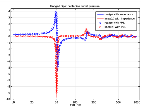
In the Settings window for 1D Plot Group, type Flanged pipe: centerline outlet pressure in the Label text field.
3
Locate the Data section. From the Dataset list, choose None.
4
Locate the Title section. From the Title type list, choose Label.
Point Graph 1
1
Right-click Flanged pipe: centerline outlet pressure and choose Point Graph.
2
In the Settings window for Point Graph, locate the Data section.
3
From the Dataset list, choose Study 1 - Flanged pipe with impedance BC/Solution 1 (sol1).
4
5
Locate the y-Axis Data section. In the Expression text field, type real(acpr.p_t).
6
Locate the Coloring and Style section. From the Color list, choose Blue.
7
Locate the Legends section. Select the Show legends check box.
8
From the Legends list, choose Manual.
9
10
In the Flanged pipe: centerline outlet pressure toolbar, click  Plot.
Point Graph 2
1
In the Model Builder window, right-click Flanged pipe: centerline outlet pressure and choose Point Graph.
2
In the Settings window for Point Graph, locate the Data section.
3
From the Dataset list, choose Study 1 - Flanged pipe with impedance BC/Solution 1 (sol1).
4
Locate the y-Axis Data section. In the Expression text field, type imag(acpr.p_t).
5
Locate the Coloring and Style section. From the Color list, choose Red.
6
Locate the Legends section. Select the Show legends check box.
7
From the Legends list, choose Manual.
8
9
In the Flanged pipe: centerline outlet pressure toolbar, click  Plot.
10
Locate the Selection section. Click to select the  Activate Selection toggle button.
11
12
In the Flanged pipe: centerline outlet pressure toolbar, click  Plot.
Point Graph 3
1
Right-click Flanged pipe: centerline outlet pressure and choose Point Graph.
2
In the Settings window for Point Graph, locate the Data section.
3
From the Dataset list, choose Study 2 - Flanged pipe with PML/Solution 2 (sol2).
4
5
Locate the y-Axis Data section. In the Expression text field, type real(acpr2.p_t).
6
Locate the Coloring and Style section. From the Color list, choose Blue.
7
Find the Line style subsection. From the Line list, choose None.
8
Find the Line markers subsection. From the Marker list, choose Circle.
9
From the Positioning list, choose Interpolated.
10
In the Number text field, type 100.
11
Locate the Legends section. Select the Show legends check box.
12
From the Legends list, choose Manual.
13
14
In the Flanged pipe: centerline outlet pressure toolbar, click  Plot.
Point Graph 4
1
Right-click Flanged pipe: centerline outlet pressure and choose Point Graph.
2
In the Settings window for Point Graph, locate the Data section.
3
From the Dataset list, choose Study 2 - Flanged pipe with PML/Solution 2 (sol2).
4
5
Locate the y-Axis Data section. In the Expression text field, type imag(acpr2.p_t).
6
Locate the Coloring and Style section. Find the Line style subsection. From the Line list, choose None.
7
From the Color list, choose Red.
8
Find the Line markers subsection. From the Marker list, choose Circle.
9
From the Positioning list, choose Interpolated.
10
In the Number text field, type 100.
11
Locate the Legends section. Select the Show legends check box.
12
From the Legends list, choose Manual.
13
14
In the Flanged pipe: centerline outlet pressure toolbar, click  Plot.
15
Click the  x-Axis Log Scale button in the Graphics toolbar.
Now the unflanged pipe.
Unflanged pipe: centerline outlet pressure
1
In the Home toolbar, click  Add Plot Group and choose 1D Plot Group.
2
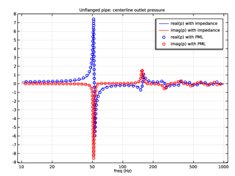
In the Settings window for 1D Plot Group, type Unflanged pipe: centerline outlet pressure in the Label text field.
3
Locate the Data section. From the Dataset list, choose None.
4
Locate the Title section. From the Title type list, choose Label.
Point Graph 1
1
Right-click Unflanged pipe: centerline outlet pressure and choose Point Graph.
2
In the Settings window for Point Graph, locate the Data section.
3
From the Dataset list, choose Study 3 - Unflanged pipe with impedance BC/Solution 3 (4) (sol3).
4
5
Locate the y-Axis Data section. In the Expression text field, type real(acpr3.p_t).
6
Locate the Coloring and Style section. From the Color list, choose Blue.
7
Locate the Legends section. Select the Show legends check box.
8
From the Legends list, choose Manual.
9
10
In the Unflanged pipe: centerline outlet pressure toolbar, click  Plot.
Point Graph 2
1
In the Model Builder window, right-click Unflanged pipe: centerline outlet pressure and choose Point Graph.
2
In the Settings window for Point Graph, locate the Data section.
3
From the Dataset list, choose Study 3 - Unflanged pipe with impedance BC/Solution 3 (4) (sol3).
4
5
Locate the y-Axis Data section. In the Expression text field, type imag(acpr3.p_t).
6
Locate the Coloring and Style section. From the Color list, choose Red.
7
Locate the Legends section. Select the Show legends check box.
8
From the Legends list, choose Manual.
9
10
In the Unflanged pipe: centerline outlet pressure toolbar, click  Plot.
Point Graph 3
1
Right-click Unflanged pipe: centerline outlet pressure and choose Point Graph.
2
In the Settings window for Point Graph, locate the Data section.
3
From the Dataset list, choose Study 4 - Unflanged pipe with PML/Solution 4 (6) (sol4).
4
5
Locate the y-Axis Data section. In the Expression text field, type real(acpr4.p_t).
6
Locate the Coloring and Style section. Find the Line style subsection. From the Line list, choose None.
7
From the Color list, choose Blue.
8
Find the Line markers subsection. From the Marker list, choose Circle.
9
From the Positioning list, choose Interpolated.
10
Locate the Legends section. Select the Show legends check box.
11
From the Legends list, choose Manual.
12
13
In the Unflanged pipe: centerline outlet pressure toolbar, click  Plot.
14
Locate the Coloring and Style section. In the Number text field, type 100.
15
In the Unflanged pipe: centerline outlet pressure toolbar, click  Plot.
Point Graph 4
1
Right-click Unflanged pipe: centerline outlet pressure and choose Point Graph.
2
In the Settings window for Point Graph, locate the Data section.
3
From the Dataset list, choose Study 4 - Unflanged pipe with PML/Solution 4 (6) (sol4).
4
5
Locate the y-Axis Data section. In the Expression text field, type imag(acpr4.p_t).
6
Locate the Coloring and Style section. Find the Line style subsection. From the Line list, choose None.
7
From the Color list, choose Red.
8
Locate the Legends section. Select the Show legends check box.
9
From the Legends list, choose Manual.
10
11
In the Unflanged pipe: centerline outlet pressure toolbar, click  Plot.
12
Locate the Coloring and Style section. Find the Line markers subsection. From the Marker list, choose Circle.
13
From the Positioning list, choose Interpolated.
14
In the Number text field, type 100.
15
In the Unflanged pipe: centerline outlet pressure toolbar, click  Plot.
16
Click the  x-Axis Log Scale button in the Graphics toolbar.
Disable the unflanged interfaces in the first two studies, so that you can run them later.
Study 1 - Flanged pipe with impedance BC
Step 1: Frequency Domain
1
In the Model Builder window, under Study 1 - Flanged pipe with impedance BC click Step 1: Frequency Domain.
2
In the Settings window for Frequency Domain, locate the Physics and Variables Selection section.
3
Study 2 - Flanged pipe with PML
Step 1: Frequency Domain
1
In the Model Builder window, under Study 2 - Flanged pipe with PML click Step 1: Frequency Domain.
2
In the Settings window for Frequency Domain, locate the Physics and Variables Selection section.
3
Solving Study 3 and Study 4 generates datasets based on the results in Component 1, where no physics is solved for. You can remove the unused datasets to clean up the model.
Results
In the Model Builder window, expand the Results>Datasets node.
Study 3 - Unflanged pipe with impedance BC/Solution 3 (3) (sol3), Study 4 - Unflanged pipe with PML/Solution 4 (5) (sol4)
1
In the Model Builder window, under Results>Datasets, Ctrl-click to select Study 3 - Unflanged pipe with impedance BC/Solution 3 (3) (sol3) and Study 4 - Unflanged pipe with PML/Solution 4 (5) (sol4).
2