PDF

Topology Optimization of a Magnetic Circuit
Introduction
This model presents an example of topology optimization of the magnetic circuit of a loudspeaker driver. Topology optimization is used to find the design of a nonlinear iron pole piece and top plate that maximize the performance, defined by a given objective, while constraining the amount of iron, obtaining a light design. The model sets up two different objectives for the optimization solved separately. The first maximized the magnetic field strength in the air gap, while the second generates a flat BL(x) curve. The final geometry features a loudspeaker that uses a smaller volume of iron and has much better characteristics than the traditional design.
The geometry and simulation parameters are similar to those used in the tutorial Loudspeaker Driver — Frequency-Domain Analysis. More insight in the vibroacoustics analysis of that geometry can be found in the documentation relative to the model.
This model illustrates:
-
-
another objective ensures a flat BL(x) curve for larger displacements of the voice coil
Model Definition
The magnetic circuit of a loudspeaker is used to concentrate the magnetic flux generated by a permanent magnet into an air gap in which a coil is placed, with the coil windings perpendicular to magnetic flux lines. The coil is mechanically connected to the membrane of the loudspeaker. When a current is run through the coil, electromagnetic forces act on it inducing movement. The movement of the coil is transferred to the membrane, which interacts with the air producing sound waves.
In a loudspeaker, the pole piece and top plate that constitute the magnetic circuit must be designed to maximize the flux concentrated at the coil, and to provide a uniform field across the coil. In order to estimate the performance of a loudspeaker magnetic circuit, it is useful to introduce the BL factor, defined as the product of magnetic flux in the air gap B and coil length L. The larger this parameter, the higher the performance of the magnetic circuit.
If the magnetic circuit is axisymmetric and the coils are winded in the azimuthal direction inside the air gap, as in the present model, the BL factor is defined as
where Br is the r-component of the magnetic flux density, N0 is the number of turns of the coil, A the cross-section area of the coil, and x is the location of voice coil. Here the BL factor will depend on the location of the voice coil, as the r-component of the magnetic flux density is not uniform for all positions of the speaker.
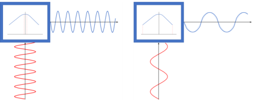
When loudspeakers are excited at high frequencies, the displacement of the membrane is always relatively small. This means that at high frequencies, the BL factor along the path of the coil is almost constant and the most relevant characteristic of the magnetic circuit is the BL factor at the resting position, that is, BL(x = 0). At low frequencies, this displacement becomes significant and the variation of the BL factor becomes more relevant. This variation of the BL factor along the path of the coil is an undesired effect as it introduces distortion in the speaker. This effect is further explained in Figure 1.
Figure 1: Lorentz force over the voice coil (blue curves along the horizontal axis) when a high frequency (left) and low frequency (right) current travels through the voice coil (red curves along the vertical axis). At high frequency the displacement of the voice coil is small, meaning that the BL factor remains almost constant through the movement, producing negligible distortion. At low frequencies, the large displacement of the coil means that the BL factor will vary along the path, producing distortion in the displacement and the sound.
For these reasons, the model includes two different optimization studies with different objectives. The first optimization study maximizes the BL factor at the resting position x = 0, making this design ideal for tweeters and loudspeakers designed for performance at high frequencies. The second optimization study minimizes the distance between the BL(x) curve and a constant value, making the magnetic circuit closer to an ideal linear speaker. This type of design is more relevant for woofers and loudspeakers intended for low frequency applications.
In the present model, the electromagnetic problem is solved using the Magnetic Fields interface. The models uses a soft iron material from the material library available in COMSOL. This material uses a B-H curve, in order to take into account magnetic saturation. In the model, it is explicitly shown that using a given magnetic B-H curve is equivalent to using a relative permeability:
(1)
Using the relative permeability instead of the B-H curve is useful for the purpose of applying topology optimization. The permeability of the design space is defined in terms of the penalized material volume factor, θp, with the formula:
(2)
(3)
Where θmin is the minimum penalized volume fraction and psimp is the SIMP exponent. The relative permeability takes the value of the permeability of air for θp = 0 and the permeability of the iron for θp = 1. The θ field depends on the control variable field θc via a Helmholtz filter. This introduces a minimum length scale for the θ field, see the Topology Optimization of an MBB Beam tutorial in the Optimization Module Application Library for more details. In this model the minimum length scale is taken as the element size. Topology optimization is performed by searching for the values of θc in the interval [0, 1] for each element in the yoke, while constraining the volume averaged value of θ. The latter is directly proportional to the volume of iron in the design, since the θ field indicates the regions consisting of iron.
In the model there is a single domain where the iron could be placed, and in both optimization setups this leads to two isolated areas of iron. These results are similar to the traditional design of a pole piece and a top plate. For this domain, the constraint is set to a volume of about 94 cm3, which is below the volume of the original geometry, of about 110 cm3. By computing the optimal shape as a function of the constraint, it is possible to derive the Pareto front giving the relationship between the value of the objective and the volume of iron in the loudspeaker.
The third study in the model takes the results from the second topology optimization and created a solid geometry from the contour. Iron properties are added to the areas (domain) with density above 0.5 and air properties on the rest. This step validates the approach used in Equation 2.
Results and Discussion
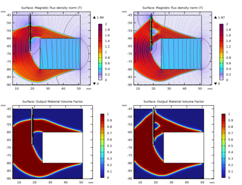
The norm of the magnetic flux density and the output material volume factor for the two optimization studies is shown in Figure 2. The left column shows the results that maximize the BL factor at the resting position; and the right column shows the results that generate a flat BL(x) curve. The figure shows that both optimization setups lead to designs consisting in two separate parts; a central component connected to the bottom of the magnet, usually called the yoke or polepiece, and a separated part connected to the top of the magnet, usually called the top plate or front plate.
Figure 2: Magnetic flux density norm (top) and Output material volume factor (bottom) for the studies maximizing the BL factor at the resting position (left) and creating a flat BL curve (right)
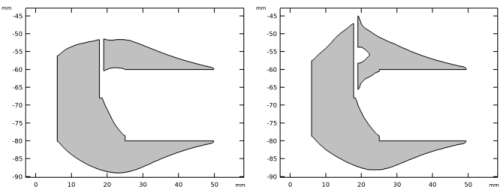
The topology optimization study produces a density map that varies between the [0,1] interval. Ideally with all of the elements in the design space should go to the minimum or the maximum density in the range. The Filter dataset transforms this density map into a geometry by removing elements (or parts of elements) with a density below a certain threshold. By choosing an intermediate density value of 0.5, it is possible to obtain a geometry that can be used to validate the B-H relation used in the topology optimization step. Figure 3 shows the geometry resulting from applying the Filter dataset to the two optimization studies.
Figure 3: Filtered results for the studies maximizing the BL factor at the resting position (left) and creating a flat BL curve (right)
The filtered results of the second optimization setup is used in a validation step, where iron properties are applied to the areas/domains with density above the threshold and air properties are applied to the rest of the design space. Figure 4 shows that the differences between the optimization model and the validation model are minimal.
As a summary, Figure 4 shows the BL(x) curve of the different models. The horizontal axis represents the voice coil offset x (the axial displacement of the voice coil) and the vertical axis represents the BL factor. The figure also includes the BL curve from a traditional design, taken from the Loudspeaker Driver — Frequency-Domain Analysis model.
Figure 4: BL Curve comparison. The plot includes the BL curve of the Optimization maximizing the BL factor at the resting position (blue), the optimization creating a flat BL curve (green), the validation model using the results from the second optimization (red), and the results of a traditional design with similar dimensions and a larger iron volume (light blue).
Notes About the COMSOL Implementation
Using the DEST() Operator TO DERIVE THE bl curve
As the coil has the same permeability as the surrounding air, the magnetic field will be equivalent for every position of the voice coil. This means that it is possible to obtain the BL curve by just averaging/integrating the B field over the different positions of the voice coil using a single stationary case. This is implemented in the model by defining an integration operation over all possible locations of the voice coil. Then, the variable coil_location_z defined as (z>(dest(z)-h_coil/2))*(z<(dest(z)+h_coil/2)) discerns whether the point should contribute to the integral or not. This logical variable will take the value of 1 when z is within the height of the coil around a given position. Note that the axial position is given by the z-coordinate in the model, while it is typically named x, hence the common name BL(x).
Using probe points to compute the Optimization objectives
The objectives of the optimizations are defined using probe points. In the first optimization, a single point at the resting position of the coil is used to obtain the BL factor and maximize it during the optimization. In the second optimization, a series of points along the path of the BL curve, given by the parameter n_points, are used to compute the squared difference between the BL(x) factor at the points (x-locations) and the objective constant BL value, given by the parameter BL_0. The optimization minimizes this squared difference, thus making the BL(x) curve as flat as possible.
Application Library path: Acoustics_Module/Optimization/magnetic_circuit_topology_optimization
Modeling Instructions
From the File menu, choose New.
New
In the New window, click  Model Wizard.
Model Wizard
1
In the Model Wizard window, click  2D Axisymmetric.
2
In the Select Physics tree, select AC/DC>Electromagnetic Fields>Magnetic Fields (mf).
3
Click Add.
4
Click  Study.
5
In the Select Study tree, select General Studies>Stationary.
6
Geometry 1
1
In the Model Builder window, under Component 1 (comp1) click Geometry 1.
2
In the Settings window for Geometry, locate the Units section.
3
From the Length unit list, choose mm.
4
In the Geometry toolbar, click Insert Sequence and choose Insert Sequence.
5
Browse to the model’s Application Libraries folder and double-click the file magnetic_circuit_topology_optimization_geom_sequence.mph.
6
In the Geometry toolbar, click  Build All.
Global Definitions
Geometry Parameters
1
In the Model Builder window, under Global Definitions click Parameters 1.
2
In the Settings window for Parameters, type Geometry Parameters in the Label text field.
Model Parameters
1
In the Home toolbar, click  Parameters and choose Add>Parameters.
2
In the Settings window for Parameters, type Model Parameters in the Label text field.
3
Locate the Parameters section. Click  Load from File.
4
Browse to the model’s Application Libraries folder and double-click the file magnetic_circuit_topology_optimization_model_parameters.txt.
Add Material
1
In the Home toolbar, click  Add Material to open the Add Material window.
2
Go to the Add Material window.
3
4
Click Add to Global Materials in the window toolbar.
5
In the tree, select AC/DC>Soft Iron (With Losses).
6
Click Add to Global Materials in the window toolbar.
7
In the Home toolbar, click  Add Material to close the Add Material window.
Global Definitions
Generic Ferrite
1
In the Model Builder window, under Global Definitions right-click Materials and choose Blank Material.
2
In the Settings window for Material, type Generic Ferrite in the Label text field.
3
Locate the Material Properties section. In the Material properties tree, select Basic Properties>Electrical Conductivity.
4
Click  Add to Material.
5
In the Material properties tree, select Basic Properties>Relative Permittivity.
6
Click  Add to Material.
7
In the Material properties tree, select Electromagnetic Models>Remanent Flux Density>Recoil permeability (murec).
8
Click  Add to Material.
9
Locate the Material Contents section. In the table, enter the following settings:
Equivalent mur of mat2, Soft Iron (With Losses)
1
In the Home toolbar, click  Functions and choose Global>Analytic.
2
In the Settings window for Analytic, type Equivalent mur of mat2, Soft Iron (With Losses) in the Label text field.
3
In the Function name text field, type mur1.
4
Locate the Definition section. In the Expression text field, type sqrt(Bx^2+By^2+eps[T^2])/mat2.BHCurve.BH_inv(sqrt(Bx^2+By^2+eps[T^2]))/mu0_const.
5
In the Arguments text field, type Bx, By.
6
Locate the Units section. In the Function text field, type 1.
7
8
Locate the Plot Parameters section. In the table, enter the following settings:
9
Definitions
Area to Obtain the BL Factor
1
In the Definitions toolbar, click  Nonlocal Couplings and choose Integration.
2
In the Settings window for Integration, type Area to Obtain the BL Factor in the Label text field.
3
In the Operator name text field, type int_BL.
4
Locate the Source Selection section. From the Selection list, choose Voice Coil Possible Locations.
5
Locate the Advanced section. In the Integration order text field, type 30.
6
Clear the Compute integral in revolved geometry check box.
Global Variables
1
In the Model Builder window, right-click Definitions and choose Variables.
2
In the Settings window for Variables, type Global Variables in the Label text field.
3
Locate the Variables section. In the table, enter the following settings:
Point Variables
1
Right-click Definitions and choose Variables.
2
In the Settings window for Variables, type Point Variables in the Label text field.
3
Locate the Geometric Entity Selection section. From the Geometric entity level list, choose Point.
4
From the Selection list, choose All points.
5
Locate the Variables section. In the table, enter the following settings:
Point Probe - Objective 1
1
In the Definitions toolbar, click  Probes and choose Point Probe.
2
In the Settings window for Point Probe, type Point Probe - Objective 1 in the Label text field.
3
In the Variable name text field, type obj_1.
4
Locate the Source Selection section. From the Selection list, choose Voice Coil Center at Resting Position.
5
Locate the Expression section. In the Expression text field, type BL_point.
Point Probe - Objective 2
1
In the Definitions toolbar, click  Probes and choose Point Probe.
2
In the Settings window for Point Probe, type Point Probe - Objective 2 in the Label text field.
3
In the Variable name text field, type obj_2.
4
Locate the Source Selection section. From the Selection list, choose Voice Coil Center Measuring Points.
5
Locate the Expression section. In the Expression text field, type (BL_point-BL_0)^2.
Component 1 (comp1)
Density Model 1 (dtopo1)
1
In the Definitions toolbar, click  Optimization and choose Topology Optimization>Density Model.
2
In the Settings window for Density Model, locate the Geometric Entity Selection section.
3
From the Selection list, choose Design Space.
4
Locate the Interpolation section. From the pSIMP list, choose User defined.
5
6
From the θmin list, choose User defined.
7
8
Locate the Control Variable Discretization section. From the Element order list, choose Constant.
9
Locate the Control Variable Initial Value section. In the θ0 text field, type volfrac.
Materials
Air
1
In the Model Builder window, under Component 1 (comp1) right-click Materials and choose More Materials>Material Link.
2
In the Settings window for Material Link, type Air in the Label text field.
Topology Optimization
1
Right-click Materials and choose More Materials>Material Link.
2
In the Settings window for Material Link, type Topology Optimization in the Label text field.
3
Locate the Geometric Entity Selection section. From the Selection list, choose Design Space.
4
Locate the Link Settings section. From the Material list, choose Soft Iron (With Losses) (mat2).
Magnet
1
Right-click Materials and choose More Materials>Material Link.
2
In the Settings window for Material Link, type Magnet in the Label text field.
3
Locate the Geometric Entity Selection section. From the Selection list, choose Magnet.
4
Locate the Link Settings section. From the Material list, choose Generic Ferrite (mat3).
Magnetic Fields (mf)
1
In the Model Builder window, under Component 1 (comp1) click Magnetic Fields (mf).
2
In the Settings window for Magnetic Fields, click to expand the Discretization section.
3
From the Magnetic vector potential list, choose Linear.
Topology Optimization
1
In the Physics toolbar, click  Domains and choose Ampère’s Law.
2
In the Settings window for Ampère’s Law, type Topology Optimization in the Label text field.
3
Locate the Domain Selection section. From the Selection list, choose Design Space.
4
Locate the Constitutive Relation B-H section. From the μr list, choose User defined. In the associated text field, type 1+dtopo1.theta_p*(mur1(mf.Br,mf.Bz)-1).
Magnet
1
In the Physics toolbar, click  Domains and choose Ampère’s Law.
2
In the Settings window for Ampère’s Law, type Magnet in the Label text field.
3
Locate the Domain Selection section. From the Selection list, choose Magnet.
4
Locate the Constitutive Relation B-H section. From the Magnetization model list, choose Remanent flux density.
5
Specify the e vector as
Mesh 1
Mapped 1
1
In the Mesh toolbar, click  Mapped.
2
In the Settings window for Mapped, locate the Domain Selection section.
3
From the Geometric entity level list, choose Domain.
4
From the Selection list, choose Mapped Domains.
Size 1
1
Right-click Mapped 1 and choose Size.
2
In the Settings window for Size, locate the Element Size section.
3
Click the Custom button.
4
Locate the Element Size Parameters section.
5
Select the Maximum element size check box. In the associated text field, type mesh_size.
Free Triangular 1
In the Mesh toolbar, click  Free Triangular.
Size 1
1
Right-click Free Triangular 1 and choose Size.
2
In the Settings window for Size, locate the Geometric Entity Selection section.
3
From the Geometric entity level list, choose Domain.
4
From the Selection list, choose Design Space.
5
Locate the Element Size section. Click the Custom button.
6
Locate the Element Size Parameters section.
7
Select the Maximum element size check box. In the associated text field, type mesh_size.
Size
1
In the Model Builder window, under Component 1 (comp1)>Mesh 1 click Size.
2
In the Settings window for Size, locate the Element Size section.
3
From the Predefined list, choose Finer.
4
Click  Build All.
Study 1 - Max BL at Rest Optimization
1
In the Model Builder window, click Study 1.
2
In the Settings window for Study, type Study 1 - Max BL at Rest Optimization in the Label text field.
Topology Optimization
1
In the Study toolbar, click  Optimization and choose Topology Optimization.
2
In the Settings window for Topology Optimization, locate the Optimization Solver section.
3
In the Maximum number of iterations text field, type 20.
4
Click Add Expression in the upper-right corner of the Objective Function section. From the menu, choose Component 1 (comp1)>Definitions>comp1.obj_1 - Point Probe - Objective 1 - Wb/m.
5
Locate the Objective Function section. From the Type list, choose Maximization.
6
From the Objective scaling list, choose Initial solution based.
7
Click Add Expression in the upper-right corner of the Constraints section. From the menu, choose Component 1 (comp1)>Definitions>Density Model 1>Global>comp1.dtopo1.theta_avg - Average material volume factor.
8
Locate the Constraints section. In the table, enter the following settings:
9
Locate the Output While Solving section. From the Probes list, choose None.
10
In the Study toolbar, click  Get Initial Value.
11
In the Model Builder window, click Topology Optimization.
12
In the Settings window for Topology Optimization, locate the Output While Solving section.
13
Select the Plot check box.
14
From the Plot group list, choose Output material volume factor.
15
In the Study toolbar, click  Compute.
Results
Revolution 2D 1
1
In the Model Builder window, expand the Results>Datasets node.
2
Right-click Results>Datasets>Revolution 2D 1 and choose Delete.
Filter - Max BL at Rest Optimization
1
In the Model Builder window, under Results>Datasets click Filter.
2
In the Settings window for Filter, type Filter - Max BL at Rest Optimization in the Label text field.
3
Locate the Expression section. In the Expression text field, type if(isnan(dtopo1.theta_c),NaN,dtopo1.theta).
Threshold
1
In the Model Builder window, expand the Results>Topology Optimization node, then click Threshold.
2
In the Threshold toolbar, click  Plot.
Magnetic Flux Density Norm (mf)
1
In the Model Builder window, under Results click Magnetic Flux Density Norm (mf).
2
In the Settings window for 2D Plot Group, locate the Plot Settings section.
3
From the View list, choose View 1.
Surface 1
1
In the Model Builder window, expand the Magnetic Flux Density Norm (mf) node, then click Surface 1.
2
In the Settings window for Surface, click to expand the Range section.
3
Select the Manual color range check box.
4
In the Minimum text field, type 0.
5
In the Maximum text field, type 2.
6
In the Magnetic Flux Density Norm (mf) toolbar, click  Plot.
Magnetic Flux Density Norm (mf)
1
In the Model Builder window, click Magnetic Flux Density Norm (mf).
2
Drag and drop on Topology Optimization.
Max BL at Rest Optimization Results
1
In the Model Builder window, under Results click Topology Optimization.
2
In the Settings window for Group, type Max BL at Rest Optimization Results in the Label text field.
Output material volume factor
1
In the Model Builder window, click Output material volume factor.
2
In the Settings window for 2D Plot Group, locate the Plot Settings section.
3
From the View list, choose View 1.
Surface 1
1
In the Model Builder window, expand the Output material volume factor node, then click Surface 1.
2
In the Settings window for Surface, locate the Expression section.
3
In the Expression text field, type if(isnan(dtopo1.theta_c),NaN,dtopo1.theta).
4
Select the Description check box. In the associated text field, type Output Material Volume Factor.
5
In the Output material volume factor toolbar, click  Plot.
Add Study
1
In the Home toolbar, click  Add Study to open the Add Study window.
2
Go to the Add Study window.
3
Find the Studies subsection. In the Select Study tree, select General Studies>Stationary.
4
Click Add Study in the window toolbar.
5
In the Home toolbar, click  Add Study to close the Add Study window.
Study 2 - Flat BL Optimization
1
In the Model Builder window, click Study 2.
2
In the Settings window for Study, type Study 2 - Flat BL Optimization in the Label text field.
Topology Optimization
1
In the Study toolbar, click  Optimization and choose Topology Optimization.
2
In the Settings window for Topology Optimization, locate the Optimization Solver section.
3
In the Maximum number of iterations text field, type 50.
4
Click Add Expression in the upper-right corner of the Objective Function section. From the menu, choose Component 1 (comp1)>Definitions>comp1.obj_2 - Point Probe - Objective 2 - kg²·m²/(s4·A²).
5
Locate the Objective Function section. From the Objective scaling list, choose Initial solution based.
6
Click Add Expression in the upper-right corner of the Constraints section. From the menu, choose Component 1 (comp1)>Definitions>Density Model 1>Global>comp1.dtopo1.theta_avg - Average material volume factor.
7
Locate the Constraints section. In the table, enter the following settings:
8
Locate the Output While Solving section. From the Probes list, choose None.
9
In the Study toolbar, click  Get Initial Value.
10
In the Model Builder window, click Topology Optimization.
11
In the Settings window for Topology Optimization, locate the Output While Solving section.
12
Select the Plot check box.
13
From the Plot group list, choose Output material volume factor 1.
14
In the Study toolbar, click  Compute.
Results
Revolution 2D 1
In the Model Builder window, under Results>Datasets right-click Revolution 2D 1 and choose Delete.
Filter - Flat BL Optimization
1
In the Model Builder window, under Results>Datasets click Filter.
2
In the Settings window for Filter, type Filter - Flat BL Optimization in the Label text field.
3
Locate the Expression section. In the Expression text field, type if(isnan(dtopo1.theta_c),NaN,dtopo1.theta).
Filter - Initial Geometry
1
Right-click Filter - Flat BL Optimization and choose Duplicate.
2
In the Settings window for Filter, type Filter - Initial Geometry in the Label text field.
3
Locate the Expression section. In the Expression text field, type 1.
Threshold 1
1
In the Model Builder window, expand the Results>Topology Optimization node, then click Threshold 1.
2
In the Settings window for 2D Plot Group, locate the Plot Settings section.
3
From the View list, choose View 1.
4
In the Threshold 1 toolbar, click  Plot.
Magnetic Flux Density Norm (mf) 1
1
In the Model Builder window, under Results click Magnetic Flux Density Norm (mf) 1.
2
In the Settings window for 2D Plot Group, locate the Plot Settings section.
3
From the View list, choose View 1.
Surface 1
1
In the Model Builder window, expand the Magnetic Flux Density Norm (mf) 1 node, then click Surface 1.
2
In the Settings window for Surface, locate the Range section.
3
Select the Manual color range check box.
4
In the Minimum text field, type 0.
5
In the Maximum text field, type 2.
6
In the Magnetic Flux Density Norm (mf) 1 toolbar, click  Plot.
Magnetic Flux Density Norm (mf) 1
1
In the Model Builder window, click Magnetic Flux Density Norm (mf) 1.
2
Drag and drop on Topology Optimization.
Flat BL Optimization Results
1
In the Model Builder window, under Results click Topology Optimization.
2
In the Settings window for Group, type Flat BL Optimization Results in the Label text field.
Output material volume factor 1
1
In the Model Builder window, click Output material volume factor 1.
2
In the Settings window for 2D Plot Group, locate the Plot Settings section.
3
From the View list, choose View 1.
Surface 1
1
In the Model Builder window, expand the Output material volume factor 1 node, then click Surface 1.
2
In the Settings window for Surface, locate the Expression section.
3
In the Expression text field, type if(isnan(dtopo1.theta_c),NaN,dtopo1.theta).
4
Select the Description check box. In the associated text field, type Output Material Volume Factor.
5
In the Output material volume factor 1 toolbar, click  Plot.
Filter - Flat BL Optimization
In the Model Builder window, under Results>Datasets right-click Filter - Flat BL Optimization and choose Create Mesh Part.
Mesh Part 1
Import 1
In the Model Builder window, under Global Definitions>Mesh Parts>Mesh Part 1 right-click Import 1 and choose Build Selected.
Results
Filter - Initial Geometry
In the Model Builder window, under Results>Datasets right-click Filter - Initial Geometry and choose Create Mesh Part.
Mesh Part 2
Import 1
In the Model Builder window, under Global Definitions>Mesh Parts>Mesh Part 2 right-click Import 1 and choose Build Selected.
Add Component
In the Model Builder window, right-click the root node and choose Add Component>2D Axisymmetric.
Geometry 2
1
In the Settings window for Geometry, locate the Units section.
2
From the Length unit list, choose mm.
Import 1 (imp1)
1
In the Home toolbar, click  Import.
2
In the Settings window for Import, locate the Import section.
3
From the Source list, choose Mesh.
4
From the Mesh list, choose Mesh Part 1.
5
Click  Build Selected.
Import 2 (imp2)
1
In the Home toolbar, click  Import.
2
In the Settings window for Import, locate the Import section.
3
From the Source list, choose Mesh.
4
From the Mesh list, choose Mesh Part 2.
5
Click  Build Selected.
Definitions (comp2)
Area to Obtain the BL Factor 2
1
In the Definitions toolbar, click  Nonlocal Couplings and choose Integration.
2
In the Settings window for Integration, type Area to Obtain the BL Factor 2 in the Label text field.
3
In the Operator name text field, type int_BL2.
4
Locate the Source Selection section. From the Selection list, choose Voice Coil Possible Locations (Import 2).
5
Locate the Advanced section. In the Integration order text field, type 30.
6
Clear the Compute integral in revolved geometry check box.
Global Variables 2
1
In the Model Builder window, right-click Definitions and choose Variables.
2
In the Settings window for Variables, type Global Variables 2 in the Label text field.
3
Locate the Variables section. In the table, enter the following settings:
Materials
Air
1
In the Model Builder window, under Component 2 (comp2) right-click Materials and choose More Materials>Material Link.
2
In the Settings window for Material Link, type Air in the Label text field.
Iron
1
Right-click Materials and choose More Materials>Material Link.
2
In the Settings window for Material Link, type Iron in the Label text field.
3
Locate the Geometric Entity Selection section. From the Selection list, choose Design Space (Import 1).
Magnet
1
Right-click Materials and choose More Materials>Material Link.
2
In the Settings window for Material Link, type Magnet in the Label text field.
3
Locate the Geometric Entity Selection section. From the Selection list, choose Magnet (Import 2).
4
Locate the Link Settings section. From the Material list, choose Generic Ferrite (mat3).
Iron (matlnk5)
1
In the Model Builder window, click Iron (matlnk5).
2
In the Settings window for Material Link, locate the Link Settings section.
3
From the Material list, choose Soft Iron (With Losses) (mat2).
Add Physics
1
In the Home toolbar, click  Add Physics to open the Add Physics window.
2
Go to the Add Physics window.
3
In the tree, select AC/DC>Electromagnetic Fields>Magnetic Fields (mf).
4
Find the Physics interfaces in study subsection. In the table, clear the Solve check boxes for Study 1 - Max BL at Rest Optimization and Study 2 - Flat BL Optimization.
5
Click Add to Component 2 in the window toolbar.
6
In the Home toolbar, click  Add Physics to close the Add Physics window.
Magnetic Fields 2 (mf2)
Iron
1
Right-click Component 2 (comp2)>Magnetic Fields 2 (mf2) and choose Ampère’s Law.
2
In the Settings window for Ampère’s Law, type Iron in the Label text field.
3
Locate the Domain Selection section. From the Selection list, choose Design Space (Import 1).
4
Locate the Constitutive Relation B-H section. From the Magnetization model list, choose B-H curve.
Magnet
1
In the Physics toolbar, click  Domains and choose Ampère’s Law.
2
In the Settings window for Ampère’s Law, type Magnet in the Label text field.
3
Locate the Domain Selection section. From the Selection list, choose Magnet (Import 2).
4
Locate the Constitutive Relation B-H section. From the Magnetization model list, choose Remanent flux density.
5
Specify the e vector as
Mesh 2
Mapped 1
1
In the Mesh toolbar, click  Mapped.
2
In the Settings window for Mapped, locate the Domain Selection section.
3
From the Geometric entity level list, choose Domain.
4
From the Selection list, choose Mapped Domains (Import 2).
Size 1
1
Right-click Mapped 1 and choose Size.
2
In the Settings window for Size, locate the Element Size section.
3
Click the Custom button.
4
Locate the Element Size Parameters section.
5
Select the Maximum element size check box. In the associated text field, type mesh_size.
Free Triangular 1
In the Mesh toolbar, click  Free Triangular.
Size 1
1
Right-click Free Triangular 1 and choose Size.
2
In the Settings window for Size, locate the Geometric Entity Selection section.
3
From the Geometric entity level list, choose Domain.
4
From the Selection list, choose Design Space (Import 1).
5
Locate the Element Size section. Click the Custom button.
6
Locate the Element Size Parameters section.
7
Select the Maximum element size check box. In the associated text field, type mesh_size.
Mesh 1
Size
In the Model Builder window, under Component 1 (comp1)>Mesh 1 right-click Size and choose Build All.
Add Study
1
In the Home toolbar, click  Add Study to open the Add Study window.
2
Go to the Add Study window.
3
Find the Studies subsection. In the Select Study tree, select General Studies>Stationary.
4
Find the Physics interfaces in study subsection. In the table, clear the Solve check box for Magnetic Fields (mf).
5
Click Add Study in the window toolbar.
6
In the Home toolbar, click  Add Study to close the Add Study window.
Study 3
Step 1: Stationary
1
In the Settings window for Stationary, click to expand the Results While Solving section.
2
From the Probes list, choose None.
3
In the Model Builder window, click Study 3.
4
In the Settings window for Study, type Study 3 - Flat BL Validation in the Label text field.
5
In the Home toolbar, click  Compute.
Results
Magnetic Flux Density Norm (mf2)
1
In the Model Builder window, expand the Results>Topology Optimization node, then click Results>Magnetic Flux Density Norm (mf2).
2
In the Settings window for 2D Plot Group, locate the Plot Settings section.
3
From the View list, choose View 1.
Surface 1
1
In the Model Builder window, expand the Magnetic Flux Density Norm (mf2) node, then click Surface 1.
2
In the Settings window for Surface, locate the Range section.
3
Select the Manual color range check box.
4
In the Minimum text field, type 0.
5
In the Maximum text field, type 2.
6
In the Magnetic Flux Density Norm (mf2) toolbar, click  Plot.
Magnetic Flux Density Norm (mf2)
1
In the Model Builder window, click Magnetic Flux Density Norm (mf2).
2
Drag and drop on Topology Optimization.
Output material volume factor 2, Threshold 2
1
In the Model Builder window, under Results>Topology Optimization, Ctrl-click to select Output material volume factor 2 and Threshold 2.
2
Flat BL Validation
1
In the Model Builder window, under Results click Topology Optimization.
2
In the Settings window for Group, type Flat BL Validation in the Label text field.
Filter, Revolution 2D 1, Study 3 - Flat BL Validation/Solution 3 (4) (sol3)
1
In the Model Builder window, under Results>Datasets, Ctrl-click to select Study 3 - Flat BL Validation/Solution 3 (4) (sol3), Revolution 2D 1, and Filter.
2
Traditional Design BL Curve
1
In the Results toolbar, click  Table.
2
In the Settings window for Table, type Traditional Design BL Curve in the Label text field.
3
Locate the Data section. Click Import.
4
Browse to the model’s Application Libraries folder and double-click the file magnetic_circuit_topology_optimization_traditional_bl.txt.
BL Factor
1
In the Results toolbar, click  1D Plot Group.
2
In the Settings window for 1D Plot Group, type BL Factor in the Label text field.
3
Locate the Plot Settings section.
4
Select the x-axis label check box. In the associated text field, type Voice coil offset (mm).
5
Select the y-axis label check box. In the associated text field, type BL factor (Wb/m).
6
Click to expand the Title section. From the Title type list, choose Label.
7
Locate the Legend section. From the Position list, choose Lower middle.
Line Graph 1
1
Right-click BL Factor and choose Line Graph.
2
In the Settings window for Line Graph, locate the Selection section.
3
From the Selection list, choose Voice Coil Center Possible Locations.
4
Locate the y-Axis Data section. In the Expression text field, type int_BL(BL_integrand*coil_location_z).
5
Locate the x-Axis Data section. From the Parameter list, choose Expression.
6
In the Expression text field, type (z-z_coil).
7
Select the Description check box. In the associated text field, type Coil Offset.
8
Click to expand the Coloring and Style section. From the Width list, choose 2.
9
Click to expand the Legends section. Select the Show legends check box.
10
Find the Include subsection. Clear the Solution check box.
11
Find the Prefix and suffix subsection. In the Prefix text field, type Max BL at Rest Optimization.
12
In the BL Factor toolbar, click  Plot.
Line Graph 2
1
Right-click Line Graph 1 and choose Duplicate.
2
In the Settings window for Line Graph, locate the Data section.
3
From the Dataset list, choose Study 2 - Flat BL Optimization/Solution 2 (sol2).
4
Locate the Legends section. Find the Prefix and suffix subsection. In the Prefix text field, type Flat BL Optimization.
5
In the BL Factor toolbar, click  Plot.
Line Graph 3
1
Right-click Line Graph 2 and choose Duplicate.
2
In the Settings window for Line Graph, locate the Data section.
3
From the Dataset list, choose Study 3 - Flat BL Validation/Solution 3 (sol3).
4
Locate the Selection section. From the Selection list, choose Voice Coil Center Possible Locations (Import 2).
5
Locate the y-Axis Data section. In the Expression text field, type int_BL2(BL_integrand*coil_location_z).
6
Locate the Legends section. Find the Prefix and suffix subsection. In the Prefix text field, type Flat BL Validation.
7
In the BL Factor toolbar, click  Plot.
Annotation 1
1
In the Model Builder window, right-click BL Factor and choose Annotation.
2
In the Settings window for Annotation, locate the Coloring and Style section.
3
Clear the Show point check box.
4
In the BL Factor toolbar, click  Plot.
Table Graph 1
1
Right-click BL Factor and choose Table Graph.
2
In the Settings window for Table Graph, locate the Data section.
3
From the Table list, choose Traditional Design BL Curve.
4
In the BL Factor toolbar, click  Plot.
5
Click to expand the Legends section. Select the Show legends check box.
6
From the Legends list, choose Manual.
7
8
Locate the Coloring and Style section. From the Width list, choose 2.
9
In the BL Factor toolbar, click  Plot.
Point Graph 1
1
Right-click BL Factor and choose Point Graph.
2
In the Settings window for Point Graph, locate the Selection section.
3
From the Selection list, choose Voice Coil Center at Resting Position.
4
Locate the y-Axis Data section. In the Expression text field, type int_BL(BL_integrand*coil_location_z).
5
Locate the x-Axis Data section. From the Parameter list, choose Expression.
6
In the Expression text field, type (z-z_coil).
7
Click to expand the Coloring and Style section. Find the Line style subsection. From the Line list, choose None.
8
From the Color list, choose Cycle (reset).
9
From the Width list, choose 5.
10
Find the Line markers subsection. From the Marker list, choose Diamond.
11
In the BL Factor toolbar, click  Plot.
Point Graph 2
1
Right-click Point Graph 1 and choose Duplicate.
2
In the Settings window for Point Graph, locate the Data section.
3
From the Dataset list, choose Study 2 - Flat BL Optimization/Solution 2 (sol2).
4
Locate the Selection section. From the Selection list, choose Voice Coil Center Measuring Points.
5
In the BL Factor toolbar, click  Plot.
6
Locate the Coloring and Style section. From the Color list, choose Custom.
7
Click Define custom colors.
8
9
Click Add to custom colors.
10
Click Show color palette only or OK on the cross-platform desktop.
11
In the BL Factor toolbar, click  Plot.
Iron Volume
1
In the Results toolbar, click  Evaluation Group.
2
In the Settings window for Evaluation Group, type Iron Volume in the Label text field.
3
Locate the Data section. From the Dataset list, choose None.
Surface Measurement 1
1
In the Iron Volume toolbar, click  Measure and choose Surface Measurement.
2
In the Settings window for Surface Measurement, locate the Data section.
3
From the Dataset list, choose Filter - Max BL at Rest Optimization.
4
Locate the Measurement Settings section. From the Unit list, choose cm^3.
5
Select the Description check box. In the associated text field, type Max BL Opt.
6
In the Iron Volume toolbar, click  Evaluate.
Iron Volume
In the Model Builder window, click Iron Volume.
Surface Measurement 2
1
In the Iron Volume toolbar, click  Measure and choose Surface Measurement.
2
In the Settings window for Surface Measurement, locate the Data section.
3
From the Dataset list, choose Filter - Flat BL Optimization.
4
Locate the Measurement Settings section. From the Unit list, choose cm^3.
5
Select the Description check box. In the associated text field, type Flat BL Opt.
6
In the Iron Volume toolbar, click  Evaluate.
Iron Volume
In the Model Builder window, click Iron Volume.
Surface Measurement 3
1
In the Iron Volume toolbar, click  Measure and choose Surface Measurement.
2
In the Settings window for Surface Measurement, locate the Data section.
3
From the Dataset list, choose Study 3 - Flat BL Validation/Solution 3 (sol3).
4
Locate the Selection section. Click to select the  Activate Selection toggle button.
5
6
Locate the Measurement Settings section. From the Unit list, choose cm^3.
7
Select the Description check box. In the associated text field, type Flat BL Validation.
8
In the Iron Volume toolbar, click  Evaluate.
Geometry Modeling Instructions
If you want to create the geometry yourself, follow these steps.
From the File menu, choose New.
New
In the New window, click  Model Wizard.
Model Wizard
1
In the Model Wizard window, click  2D Axisymmetric.
2
Geometry 1
1
In the Model Builder window, under Component 1 (comp1) click Geometry 1.
2
In the Settings window for Geometry, locate the Units section.
3
From the Length unit list, choose mm.
Global Definitions
Parameters 1
1
In the Model Builder window, under Global Definitions click Parameters 1.
2
In the Settings window for Parameters, locate the Parameters section.
3
Click  Load from File.
4
Browse to the model’s Application Libraries folder and double-click the file magnetic_circuit_topology_optimization_geom_parameters.txt.
Geometry 1
Air
1
In the Geometry toolbar, click  Rectangle.
2
In the Settings window for Rectangle, type Air in the Label text field.
3
Locate the Size and Shape section. In the Width text field, type w_air.
4
In the Height text field, type h_air.
5
Locate the Position section. In the z text field, type z_design+h_design/2-h_air/2.
6
Click  Build Selected.
Design Space with Magnet and Coil Gap
1
In the Geometry toolbar, click  Rectangle.
2
In the Settings window for Rectangle, type Design Space with Magnet and Coil Gap in the Label text field.
3
Locate the Size and Shape section. In the Width text field, type w_design.
4
In the Height text field, type h_design.
5
Locate the Position section. In the r text field, type r_design.
6
In the z text field, type z_design.
7
Click  Build Selected.
Voice Coil Gap
1
In the Geometry toolbar, click  Rectangle.
2
In the Settings window for Rectangle, type Voice Coil Gap in the Label text field.
3
Locate the Size and Shape section. In the Width text field, type w_coil+w_gap_i+w_gap_o.
4
In the Height text field, type h_coil+2*z_offset.
5
Locate the Position section. In the r text field, type r_coil-w_gap_i-w_coil/2.
6
In the z text field, type z_coil-h_coil/2-z_offset.
7
Click  Build Selected.
Design Space with Magnet
1
In the Geometry toolbar, click  Booleans and Partitions and choose Difference.
2
In the Settings window for Difference, type Design Space with Magnet in the Label text field.
3
4
Locate the Difference section. Find the Objects to subtract subsection. Click to select the  Activate Selection toggle button.
5
6
Locate the Selections of Resulting Entities section. Select the Resulting objects selection check box.
7
Click  Build Selected.
Magnet
1
In the Geometry toolbar, click  Rectangle.
2
In the Settings window for Rectangle, type Magnet in the Label text field.
3
Locate the Size and Shape section. In the Width text field, type w_magnet.
4
In the Height text field, type h_magnet.
5
Locate the Position section. In the r text field, type r_magnet.
6
In the z text field, type z_magnet.
7
Locate the Selections of Resulting Entities section. Select the Resulting objects selection check box.
8
Click  Build Selected.
Voice Coil Possible Locations
1
In the Geometry toolbar, click  Rectangle.
2
In the Settings window for Rectangle, type Voice Coil Possible Locations in the Label text field.
3
Locate the Size and Shape section. In the Width text field, type w_coil.
4
In the Height text field, type h_coil+2*z_offset.
5
Locate the Position section. From the Base list, choose Center.
6
In the r text field, type r_coil.
7
In the z text field, type z_coil.
8
Click to expand the Layers section. In the table, enter the following settings:
9
Select the Layers on top check box.
10
Locate the Selections of Resulting Entities section. Select the Resulting objects selection check box.
11
Click  Build Selected.
Voice Coil Center Possible Locations
1
In the Geometry toolbar, click  More Primitives and choose Line Segment.
2
In the Settings window for Line Segment, type Voice Coil Center Possible Locations in the Label text field.
3
Locate the Starting Point section. From the Specify list, choose Coordinates.
4
In the r text field, type r_coil.
5
In the z text field, type z_coil-z_offset.
6
Locate the Endpoint section. From the Specify list, choose Coordinates.
7
In the r text field, type r_coil.
8
In the z text field, type z_coil+z_offset.
9
Locate the Selections of Resulting Entities section. Select the Resulting objects selection check box.
10
Click  Build Selected.
Lowest Voice Coil Center Point
1
In the Geometry toolbar, click  Point.
2
In the Settings window for Point, type Lowest Voice Coil Center Point in the Label text field.
3
Locate the Point section. In the r text field, type r_coil.
4
In the z text field, type z_coil-z_offset.
5
Click  Build Selected.
Voice Coil Center Measuring Points
1
In the Geometry toolbar, click  Transforms and choose Array.
2
In the Settings window for Array, type Voice Coil Center Measuring Points in the Label text field.
3
4
Locate the Size section. In the z size text field, type n_points.
5
Locate the Displacement section. In the z text field, type 2*z_offset/(n_points-1).
6
Locate the Selections of Resulting Entities section. Select the Resulting objects selection check box.
7
From the Show in physics list, choose Point selection.
8
Click  Build Selected.
Voice Coil Center at Resting Position
1
In the Geometry toolbar, click  Point.
2
In the Settings window for Point, type Voice Coil Center at Resting Position in the Label text field.
3
Locate the Point section. In the r text field, type r_coil.
4
In the z text field, type z_coil.
5
Locate the Selections of Resulting Entities section. Select the Resulting objects selection check box.
6
Click  Build Selected.
Form Union (fin)
1
In the Model Builder window, click Form Union (fin).
2
In the Settings window for Form Union/Assembly, click  Build Selected.
Mapped Domains
1
In the Geometry toolbar, click  Selections and choose Union Selection.
2
In the Settings window for Union Selection, type Mapped Domains in the Label text field.
3
Locate the Input Entities section. Click  Add.
4
In the Add dialog box, in the Selections to add list, choose Magnet and Voice Coil Possible Locations.
5
Design Space
1
In the Geometry toolbar, click  Selections and choose Difference Selection.
2
In the Settings window for Difference Selection, type Design Space in the Label text field.
3
Locate the Input Entities section. Click  Add.
4
In the Add dialog box, select Design Space with Magnet in the Selections to add list.
5
6
In the Settings window for Difference Selection, locate the Input Entities section.
7
8
In the Add dialog box, select Magnet in the Selections to subtract list.
9