PDF

Helmholtz Resonator with Flow:
Interaction of Flow and Acoustics
Introduction
Helmholtz resonators are used in exhaust systems as they can attenuate a specific narrow frequency band. The presence of a flow in the system alters the acoustic properties of the resonator and hence the transmission loss of the subsystem. In this model example a Helmholtz resonator is located as a side branch to a main duct. The transmission loss through the main duct is investigated when a mean flow is introduced.
The mean background flow in the system is calculated with the SST turbulence model for Mach numbers Ma = 0.05 and Ma = 0.1. The acoustic problem is then solved using the Linearized Navier-Stokes, Frequency Domain (LNS) physics interface. The mean flow velocity, pressure, and turbulent viscosity are coupled to the LNS model using the Background Fluid Flow Coupling multiphysics feature. The dedicated mapping study is used to interpolate the flow solution from the CFD mesh onto the acoustics mesh. The no-flow case is solved using Pressure Acoustics, Frequency Domain.
The geometry dimensions of the system are taken from those presented in Ref. 1. The results can be compared to the measurements found in the journal paper.
Note: This model requires both the Acoustics Module and the CFD Module.
Model Definition
The geometry and dimensions are the same as the ones presented in Ref. 1. The geometry consists of a main cylindrical duct with a diameter of 4.859 cm and a Helmholtz resonator attached to the side. The resonator has a neck of length 8.05 cm and diameter 4.044 cm. The volume of the resonator is 4501 cm3. The geometry is depicted in Figure 1. The symmetry of the system has been utilized.
The system is filled with air. A mean stationary background flow of average velocity Uin = c0·Ma enters at the left (downstream in the z-axis orientation), where c0 is the speed of sound. Three flow configurations are studied with Ma = 0 (no flow), Ma = 0.05, and Ma = 0.1.
A plane acoustic wave enters the system downstream. The wave is added as a Background Acoustics Field feature in a small domain backed with a perfectly matched layer (PML). In this way, reflected waves are free to leave the computational domain both downstream and upstream. A PML is also added at the upstream outlet. The background plane wave variables are defined according to
The plane wave expressions are imported into variables in the model. Since the acoustics are solved using the linearized Navier–Stokes equations, perturbations in pressure, velocity, and temperature need to be defined. These are also solved for.
Figure 1: Geometry of the Helmholtz resonator model.
The transmission loss of the system is defined as
where pout is the average pressure at the outlet and the incident field is defined with an amplitude of 1 Pa.
Two effects are important to capture correctly when analyzing this kind of system. It is the attenuation experience by the acoustic field as it interacts with turbulence (see Ref. 2 and Ref. 3) and the convective effects of the flow and the interaction with the flow gradients. The two phenomena have opposite effects on the resonance frequency of the system. The additional attenuation due to turbulence will shift the resonance toward a lower frequency while the convective flow effects will shift it to a higher frequency. If the two are not correctly captured the results will be wrong. The transmission loss calculation is a good indicator that this is done correctly; this is seen in Figure 8 below. In order to capture the turbulence attenuation in detail, the SST turbulence model is used for the CFD as it introduces much less numerical diffusion and gives a better prediction of the eddy viscosity. The detailed interaction between flow and acoustics including the extra attenuation can only be modeled using the linearized Navier-Stokes equations as available in the Acoustics Module.
Results and Discussion
The magnitude of the mean background flow velocity is depicted in Figure 2 and the turbulent viscosity is depicted in Figure 3. The value of the turbulent viscosity should be compared to the dynamic viscosity of air μ = 2·10-5 Pa·s. At the highest Mach number (depicted in the figure) the resulting experienced viscosity will be a factor 200 larger than the no-flow situation.
Figure 2: Background mean flow velocity magnitude for Ma = 0.1.
Figure 3: Turbulent viscosity for Ma = 0.1.
When the Background Fluid Flow Coupling and the Mapping study is used, it is good practice to visualize the mapped solution and compare it to the original solution on the CFD mesh. In Figure 4 the axial flow velocity and the turbulent viscosity evaluated on the CFD mesh is compared to the mapped values on the acoustics mesh.
Figure 4: Mapped value of the axial velocity (left) and turbulent viscosity (right) compared to the value as evaluated on the CFD mesh: dashed and solid curves, respectively.
The total acoustic pressure in the system is depicted at 150 Hz for the three cases, no flow in Figure 5, Ma = 0.05 in Figure 6, and Ma = 0.1 in Figure 7.
Figure 5: Acoustic pressure in the no flow situation (Ma = 0).
Figure 6: Acoustic pressure for Ma = 0.05.
Figure 7: Acoustic pressure for Ma = 0.1.
Finally, the transmission loss of the system is depicted in Figure 8. The graph can be compared to measurements performed on the same system presented in Ref. 1. The results show good agreement.
Figure 8: Transmission loss for the three flow configurations.
Notes About the COMSOL Implementation
Mapping between CFD and Acoustics
The mapping of the fluid flow solution from the CFD mesh to the acoustics mesh is achieved using the built-in Background Fluid Flow Coupling multiphysics feature and the dedicated Mapping study.
CFD model notes
It is a common practice to use an already computed CFD solution as the initial solution while incrementing the Mach number, which results in a better convergence of the nonlinear problem. That is, the solution obtained for Ma = 0.05 will be used as the initial solution at Ma = 0.1 in this model.
This technique is achieved as follows:
Check the Auxiliary sweep check box available in the Study Extensions section of the corresponding study and specify the desired values of the flow Mach number parameter.
Choose No parameter from the Run continuation for list.
Select Yes from the Reuse solution from previous step list.
References
1. E. Selamet, A. Selamet, A. Iqbal, and H. Kim, “Effect of Flow in Helmholtz Resonator Acoustics: A Three-Dimensional Computational Study vs. Experiments,” SAE Technical Paper 2011-01-1521, SAE Int. J., 2011.
2. L. Du, A. Holmberg, M. Karlsson, and M Åbom, “Sound amplification at a rectangular T-junction with merging mean flows,” J. Sound Vib., vol. 367, pp. 69–83 2016.
3. J. Gikadi, S. Föller, and T. Sattelmayer, “Impact of turbulence on the prediction of linear aerodynamic interactions: Acoustic response of a turbulent shear layer,” J. Sound Vib., vol. 333, pp. 6548–6559, 2014.
Application Library path: Acoustics_Module/Aeroacoustics_and_Noise/helmholtz_resonator_with_flow
Modeling Instructions
The following model consists of several steps. First the background mean flow is solved using the CFD Module, then the CFD solution is mapped to the acoustics mesh using the multiphysics coupling and the mapping study, then the acoustics is solved with the mapped flow as input, finally the results are postprocessed.
The first step is to set up the CFD model and solve the flow for two Mach numbers. Running this part of the model can take about 5 h.
From the File menu, choose New.
New
In the New window, click  Model Wizard.
Model Wizard
1
In the Model Wizard window, click  3D.
2
In the Select Physics tree, select Fluid Flow>Single-Phase Flow>Turbulent Flow>Turbulent Flow, SST (spf).
3
Click Add.
4
Click  Study.
5
In the Select Study tree, select Preset Studies for Selected Physics Interfaces>Stationary with Initialization.
6
Global Definitions
In the Model Builder window, collapse the Global Definitions node.
Parameters 1
1
In the Model Builder window, under Global Definitions click Parameters 1.
2
In the Settings window for Parameters, locate the Parameters section.
3
Click  Load from File.
4
The first step is to build the geometry of the Helmholtz resonator system. To save time you can Insert Sequence from file by referring to the helmholtz_renoator_with_flow.mph file in the applications folder of the COMSOL installation.
Geometry 1
Cylinder 1 (cyl1)
1
In the Geometry toolbar, click  Cylinder.
2
In the Settings window for Cylinder, locate the Size and Shape section.
3
In the Radius text field, type Dmain/2.
4
In the Height text field, type Lin+Lout+2*Lpml.
5
Locate the Position section. In the z text field, type -Lin-Lpml.
6
Click to expand the Layers section. In the table, enter the following settings:
7
Clear the Layers on side check box.
8
Select the Layers on bottom check box.
9
Select the Layers on top check box.
Cylinder 2 (cyl2)
1
In the Geometry toolbar, click  Cylinder.
2
In the Settings window for Cylinder, locate the Size and Shape section.
3
In the Radius text field, type Dneck/2.
4
In the Height text field, type 1.2*Lneck.
5
Locate the Position section. In the x text field, type Dmain/2-0.2*Lneck.
6
Locate the Axis section. From the Axis type list, choose x-axis.
Cylinder 3 (cyl3)
1
In the Geometry toolbar, click  Cylinder.
2
In the Settings window for Cylinder, locate the Size and Shape section.
3
In the Radius text field, type Dreson/2.
4
In the Height text field, type Lreson.
5
Locate the Position section. In the x text field, type Dmain/2+Lneck.
6
Locate the Axis section. From the Axis type list, choose x-axis.
Cylinder 4 (cyl4)
1
In the Geometry toolbar, click  Cylinder.
2
In the Settings window for Cylinder, locate the Size and Shape section.
3
In the Radius text field, type Dmain/2.
4
In the Height text field, type Lsource.
5
Locate the Position section. In the z text field, type -Lin.
Cylinder 5 (cyl5)
1
In the Geometry toolbar, click  Cylinder.
2
In the Settings window for Cylinder, locate the Size and Shape section.
3
In the Radius text field, type Dmain/2.
4
In the Height text field, type 0.2.
5
Locate the Position section. In the z text field, type -0.1.
6
Click  Build Selected.
Partition Domains 1 (pard1)
1
In the Geometry toolbar, click  Booleans and Partitions and choose Partition Domains.
2
On the object cyl2, select Domain 1 only.
3
In the Settings window for Partition Domains, locate the Partition Domains section.
4
From the Partition with list, choose Extended faces.
5
On the object cyl1, select Boundaries 12 and 15 only.
It might be easier to select the boundaries by using the Selection List window. To open this window, in the Home toolbar click Windows and choose Selection List. (If you are running the cross-platform desktop, you find Windows in the main menu.)
6
From the Repair tolerance list, choose Relative.
7
Click  Build All Objects.
8
Click the  Wireframe Rendering button in the Graphics toolbar.
Delete Entities 1 (del1)
1
In the Model Builder window, right-click Geometry 1 and choose Delete Entities.
2
In the Settings window for Delete Entities, locate the Entities or Objects to Delete section.
3
From the Geometric entity level list, choose Domain.
4
On the object pard1, select Domain 1 only.
5
Click  Build Selected.
Union 1 (uni1)
1
In the Geometry toolbar, click  Booleans and Partitions and choose Union.
2
Click in the Graphics window and then press Ctrl+A to select all objects.
Work Plane 1 (wp1)
1
In the Geometry toolbar, click  Work Plane.
2
In the Settings window for Work Plane, locate the Plane Definition section.
3
From the Plane list, choose zx-plane.
Partition Objects 1 (par1)
1
In the Geometry toolbar, click  Booleans and Partitions and choose Partition Objects.
2
3
In the Settings window for Partition Objects, locate the Partition Objects section.
4
From the Partition with list, choose Work plane.
5
Click  Build Selected.
Delete Entities 2 (del2)
1
Right-click Geometry 1 and choose Delete Entities.
2
In the Settings window for Delete Entities, locate the Entities or Objects to Delete section.
3
From the Geometric entity level list, choose Domain.
4
On the object par1, select Domains 2, 4, 6, 8, 10, 12, 14, and 16 only.
5
Click  Build All Objects.
Rotate the geometry in the Graphics window. The geometry should look like the figure above.
Symmetry
1
In the Definitions toolbar, click  Explicit.
2
In the Settings window for Explicit, locate the Input Entities section.
3
From the Geometric entity level list, choose Boundary.
4
5
In the Label text field, type Symmetry.
Walls
1
In the Definitions toolbar, click  Explicit.
2
In the Settings window for Explicit, locate the Input Entities section.
3
From the Geometric entity level list, choose Boundary.
4
5
In the Label text field, type Walls.
Add Material
1
In the Home toolbar, click  Add Material to open the Add Material window.
2
Go to the Add Material window.
3
4
Click Add to Component in the window toolbar.
5
In the Home toolbar, click  Add Material to close the Add Material window.
Turbulent Flow, SST (spf)
1
In the Model Builder window, under Component 1 (comp1) click Turbulent Flow, SST (spf).
2
In the Settings window for Turbulent Flow, SST, locate the Physical Model section.
3
From the Compressibility list, choose Compressible flow (Ma<0.3).
The background flow is now set to be fully compressible. This results in the density to vary spatially. The effects of a non-constant background density are included in the linearized Navier-Stokes equations. The importance of including this depends on the specific application.
Symmetry 1
1
In the Physics toolbar, click  Boundaries and choose Symmetry.
2
In the Settings window for Symmetry, locate the Boundary Selection section.
3
From the Selection list, choose Symmetry.
Outlet 1
1
In the Physics toolbar, click  Boundaries and choose Outlet.
2
Inlet 1
1
In the Physics toolbar, click  Boundaries and choose Inlet.
2
3
In the Settings window for Inlet, locate the Boundary Condition section.
4
From the list, choose Fully developed flow.
5
Locate the Fully Developed Flow section. In the Uav text field, type Uin.
This boundary condition ensures a fully developed turbulent flow profile at the inlet.
Generate the mesh used for the CFD simulation. In this model, we set up a user-defined mesh consisting of hexahedral elements in the main part of the duct. Such a mesh will give the smallest amount of numerical diffusion. The turbulent viscosity will yield a good estimate of the eddy viscosity used in the acoustics model.
Mesh - CFD
1
In the Model Builder window, under Component 1 (comp1) click Mesh 1.
2
In the Settings window for Mesh, type Mesh - CFD in the Label text field.
Free Quad 1
1
In the Mesh toolbar, click  Boundary and choose Free Quad.
2
Size 1
1
Right-click Free Quad 1 and choose Size.
2
In the Settings window for Size, locate the Element Size section.
3
From the Calibrate for list, choose Fluid dynamics.
4
From the Predefined list, choose Extremely fine.
Size
1
In the Model Builder window, under Component 1 (comp1)>Mesh - CFD click Size.
2
In the Settings window for Size, locate the Element Size section.
3
From the Calibrate for list, choose Fluid dynamics.
4
Click the Custom button.
5
Locate the Element Size Parameters section. In the Maximum element size text field, type 0.005.
6
In the Minimum element size text field, type 0.001.
7
In the Maximum element growth rate text field, type 1.1.
8
In the Curvature factor text field, type 0.4.
9
In the Resolution of narrow regions text field, type 1.
Swept 1
1
In the Mesh toolbar, click  Swept.
2
In the Settings window for Swept, locate the Domain Selection section.
3
From the Geometric entity level list, choose Domain.
4
Distribution 1
1
Right-click Swept 1 and choose Distribution.
2
3
In the Settings window for Distribution, locate the Distribution section.
4
In the Number of elements text field, type 8.
Distribution 2
1
In the Model Builder window, right-click Swept 1 and choose Distribution.
2
Swept 2
1
In the Mesh toolbar, click  Swept.
2
In the Settings window for Swept, locate the Domain Selection section.
3
From the Geometric entity level list, choose Domain.
4
Distribution 1
1
Right-click Swept 2 and choose Distribution.
2
In the Settings window for Distribution, locate the Distribution section.
3
From the Distribution type list, choose Predefined.
4
In the Number of elements text field, type 50.
5
In the Element ratio text field, type 4.
6
Select the Reverse direction check box.
Swept 3
1
In the Mesh toolbar, click  Swept.
2
In the Settings window for Swept, locate the Domain Selection section.
3
From the Geometric entity level list, choose Domain.
4
Distribution 1
1
Right-click Swept 3 and choose Distribution.
2
In the Settings window for Distribution, locate the Distribution section.
3
In the Number of elements text field, type 8.
Swept 4
1
In the Mesh toolbar, click  Swept.
2
In the Settings window for Swept, locate the Domain Selection section.
3
From the Geometric entity level list, choose Domain.
4
Distribution 1
1
Right-click Swept 4 and choose Distribution.
2
In the Settings window for Distribution, locate the Distribution section.
3
From the Distribution type list, choose Predefined.
4
In the Number of elements text field, type 50.
5
In the Element ratio text field, type 4.
6
Select the Reverse direction check box.
Corner Refinement 1
1
In the Mesh toolbar, click  More Attributes and choose Corner Refinement.
2
In the Settings window for Corner Refinement, locate the Boundary Selection section.
3
From the Selection list, choose Walls.
Free Tetrahedral 1
In the Mesh toolbar, click  Free Tetrahedral.
Size 1
1
Right-click Free Tetrahedral 1 and choose Size.
2
In the Settings window for Size, locate the Geometric Entity Selection section.
3
From the Geometric entity level list, choose Boundary.
4
5
Locate the Element Size section. Click the Custom button.
6
Locate the Element Size Parameters section.
7
Select the Maximum element size check box. In the associated text field, type 0.0015.
Boundary Layers 1
In the Mesh toolbar, click  Boundary Layers.
Boundary Layer Properties
1
In the Model Builder window, click Boundary Layer Properties.
2
In the Settings window for Boundary Layer Properties, locate the Geometric Entity Selection section.
3
From the Selection list, choose Walls.
4
Locate the Layers section. In the Thickness adjustment factor text field, type 1.4.
5
Click  Build All.
The CFD mesh should look like the figure above.
Study 1 - CFD
1
In the Model Builder window, click Study 1.
2
In the Settings window for Study, type Study 1 - CFD in the Label text field.
3
Locate the Study Settings section. Clear the Generate default plots check box.
Step 2: Stationary
1
In the Model Builder window, under Study 1 - CFD click Step 2: Stationary.
2
In the Settings window for Stationary, click to expand the Study Extensions section.
3
Select the Auxiliary sweep check box.
4
5
6
From the Run continuation for list, choose Last parameter.
Enabling this option ensures that the solution obtained at Ma = 0.05 is used as the initial solution for Ma = 0.1, which results in a better convergence of the nonlinear solver.
Solution 1 (sol1)
1
In the Study toolbar, click  Show Default Solver.
After generating the solver sequence you can inspect the setup and make changes to the defaults if necessary.
Note that solving the model can take 5 h per value of the Mach number parameter (depending on your hardware).
2
Click  Compute.
Results
Cut Line 3D 1
1
In the Model Builder window, expand the Results node.
2
Right-click Results>Datasets and choose Cut Line 3D.
3
In the Settings window for Cut Line 3D, locate the Line Data section.
4
In row Point 1, set y to -0.0001.
5
In row Point 1, set z to -1.
6
In row Point 2, set x to 0.
7
In row Point 2, set y to -0.0001.
8
In row Point 2, set z to 1.
CFD: Velocity
1
In the Results toolbar, click  3D Plot Group.
2
In the Settings window for 3D Plot Group, type CFD: Velocity in the Label text field.
Volume 1
Right-click CFD: Velocity and choose Volume.
Transparency 1
In the Model Builder window, right-click Volume 1 and choose Transparency.
Streamline 1
1
In the Model Builder window, right-click CFD: Velocity and choose Streamline.
2
In the Settings window for Streamline, locate the Streamline Positioning section.
3
In the Number text field, type 50.
4
5
Click to expand the Inherit Style section. From the Plot list, choose Volume 1.
Color Expression 1
1
Right-click Streamline 1 and choose Color Expression.
2
In the CFD: Velocity toolbar, click  Plot.
The plot should reproduce Figure 2.
CFD: Turbulent Viscosity
1
In the Home toolbar, click  Add Plot Group and choose 3D Plot Group.
2
In the Settings window for 3D Plot Group, type CFD: Turbulent Viscosity in the Label text field.
Surface 1
1
Right-click CFD: Turbulent Viscosity and choose Surface.
2
In the Settings window for Surface, locate the Expression section.
3
In the Expression text field, type spf.muT.
4
In the CFD: Turbulent Viscosity toolbar, click  Plot.
The plot should reproduce Figure 3.
CFD: Turbulent Viscosity Axial
1
In the Home toolbar, click  Add Plot Group and choose 1D Plot Group.
2
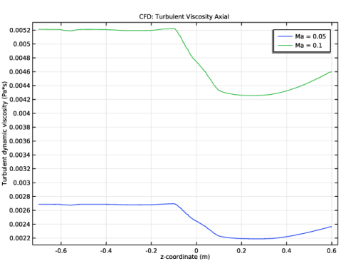
In the Settings window for 1D Plot Group, type CFD: Turbulent Viscosity Axial in the Label text field.
3
Locate the Data section. From the Dataset list, choose Cut Line 3D 1.
4
Click to expand the Title section. From the Title type list, choose Label.
CFD: Turbulent Viscosity Axial
1
Right-click CFD: Turbulent Viscosity Axial and choose Line Graph.
2
In the Settings window for Line Graph, type CFD: Turbulent Viscosity Axial in the Label text field.
3
Locate the y-Axis Data section. In the Expression text field, type spf.muT.
4
Locate the x-Axis Data section. From the Parameter list, choose Expression.
5
In the Expression text field, type z.
6
Click to expand the Legends section. Select the Show legends check box.
7
From the Legends list, choose Evaluated.
8
In the Legend text field, type Ma = eval(Ma).
9
In the CFD: Turbulent Viscosity Axial toolbar, click  Plot.
The plot shows the turbulent viscosity along the central axis of the model.
Mapping, Multiphysics, and Acoustics
An important part of solving aeroacoustic problems is to correctly map the CFD solution onto the acoustics domain. This is done using the built-in Background Fluid Flow Coupling multiphysics feature and the dedicated Mapping study.
First, add the linearized Navier-Stokes physics, then the multiphysics coupling, create a mesh for the acoustics problem, and then compute the mapping study.
Add Physics
1
In the Home toolbar, click  Add Physics to open the Add Physics window.
2
Go to the Add Physics window.
3
In the tree, select Acoustics>Aeroacoustics>Linearized Navier-Stokes, Frequency Domain (lnsf).
4
Find the Physics interfaces in study subsection. In the table, clear the Solve check box for Study 1 - CFD.
5
Click Add to Component 1 in the window toolbar.
6
In the Home toolbar, click  Add Physics to close the Add Physics window.
Multiphysics
Background Fluid Flow Coupling 1 (bffc1)
1
In the Physics toolbar, click  Multiphysics Couplings and choose Domain>Background Fluid Flow Coupling.
2
In the Settings window for Background Fluid Flow Coupling, locate the Domain Selection section.
3
From the Selection list, choose All domains.
4
Locate the Variables to Map section. Select the Map the turbulent viscosity check box.
Create the acoustics mesh that the CFD solution is mapped onto. The mesh can be relatively coarse. Note that the finer the mesh the less damping is introduced by the stabilization, this is present to stabilize sub-mesh physical phenomena like vorticity waves. At the walls we do not resolve the acoustic boundary layer since slip (and adiabatic) conditions are used here. One or two boundary layer mesh elements is enough to resolve the background flow profile near the wall.
Mesh - Acoustics
1
In the Mesh toolbar, click Add Mesh and choose Add Mesh.
2
In the Settings window for Mesh, type Mesh - Acoustics in the Label text field.
Free Tetrahedral 1
In the Mesh toolbar, click  Free Tetrahedral.
Size
1
In the Model Builder window, click Size.
2
In the Settings window for Size, locate the Element Size section.
3
Click the Custom button.
4
Locate the Element Size Parameters section. In the Maximum element size text field, type Dmain/8.
5
In the Minimum element size text field, type Dmain/15.
Free Tetrahedral 1
1
In the Model Builder window, click Free Tetrahedral 1.
2
In the Settings window for Free Tetrahedral, locate the Domain Selection section.
3
From the Geometric entity level list, choose Domain.
4
Add a Size feature to the opening of the resonator, as the flow is likely to have large gradients there.
Size 1
1
Right-click Free Tetrahedral 1 and choose Size.
2
In the Settings window for Size, locate the Geometric Entity Selection section.
3
From the Geometric entity level list, choose Boundary.
4
5
Locate the Element Size section. Click the Custom button.
6
Locate the Element Size Parameters section.
7
Select the Maximum element size check box. In the associated text field, type Dmain/15.
8
Click  Build Selected.
Swept 1
In the Mesh toolbar, click  Swept.
Distribution 1
1
Right-click Swept 1 and choose Distribution.
2
In the Settings window for Distribution, locate the Distribution section.
3
In the Number of elements text field, type 16.
4
Click  Build Selected.
Boundary Layers 1
1
In the Mesh toolbar, click  Boundary Layers.
2
In the Settings window for Boundary Layers, click to expand the Transition section.
3
Clear the Smooth transition to interior mesh check box.
Boundary Layer Properties
1
In the Model Builder window, click Boundary Layer Properties.
2
In the Settings window for Boundary Layer Properties, locate the Geometric Entity Selection section.
3
From the Selection list, choose Walls.
4
Locate the Layers section. In the Number of layers text field, type 2.
5
From the Thickness specification list, choose First layer.
6
In the Thickness text field, type Dmain/40.
7
Click  Build All.
The acoustics mesh should look like the figure above.
Add Study
1
In the Home toolbar, click  Add Study to open the Add Study window.
2
Go to the Add Study window.
3
Find the Physics interfaces in study subsection. In the table, clear the Solve check boxes for Turbulent Flow, SST (spf) and Linearized Navier-Stokes, Frequency Domain (lnsf).
4
Find the Studies subsection. In the Select Study tree, select Preset Studies for Selected Multiphysics>Mapping.
5
Click Add Study in the window toolbar.
6
In the Home toolbar, click  Add Study to close the Add Study window.
Study 2
Step 1: Mapping
1
In the Settings window for Mapping, locate the Solution to Map section.
2
From the Study list, choose Study 1 - CFD, Stationary.
3
From the Solution list, choose Solution 1 (sol1).
4
From the Parameter value (Ma) list, choose Automatic (all solutions).
Expand the Mesh Selection section to verify that the destination mesh is selected.
5
Click to expand the Destination Mesh Selection section. In the Model Builder window, click Study 2.
6
In the Settings window for Study, type Study 2 - Mapping in the Label text field.
7
In the Home toolbar, click  Compute.
Create two plots that compare the original CFD solution (evaluated on the CFD mesh) with the mapped solution (evaluated on the acoustics mesh).
Results
Mapping Comparison: z velocity
1
In the Home toolbar, click  Add Plot Group and choose 1D Plot Group.
2
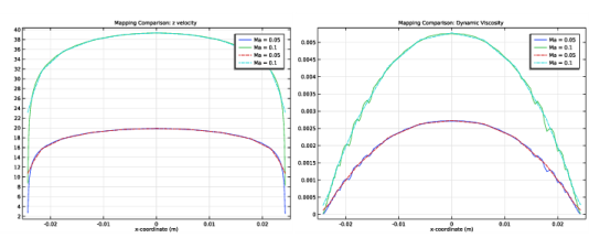
In the Settings window for 1D Plot Group, type Mapping Comparison: z velocity in the Label text field.
3
Locate the Title section. From the Title type list, choose Label.
Line Graph 1
1
Right-click Mapping Comparison: z velocity and choose Line Graph.
2
In the Settings window for Line Graph, locate the Selection section.
3
Click to select the  Activate Selection toggle button.
4
5
Locate the y-Axis Data section. In the Expression text field, type w.
6
Locate the x-Axis Data section. From the Parameter list, choose Expression.
7
In the Expression text field, type x.
8
Locate the Legends section. Select the Show legends check box.
9
From the Legends list, choose Evaluated.
10
In the Legend text field, type Ma = eval(Ma).
Line Graph 2
1
In the Model Builder window, right-click Mapping Comparison: z velocity and choose Line Graph.
2
In the Settings window for Line Graph, locate the Data section.
3
From the Dataset list, choose Study 2 - Mapping/Solution 3 (sol3).
4
5
Click Replace Expression in the upper-right corner of the y-Axis Data section. From the menu, choose Component 1 (comp1)>Background Fluid Flow Coupling 1>Mapped velocity - m/s>bffc1.u_mapz - Mapped velocity, z-component.
6
Locate the x-Axis Data section. From the Parameter list, choose Expression.
7
In the Expression text field, type x.
8
Click to expand the Coloring and Style section. Find the Line style subsection. From the Line list, choose Dashed.
9
Locate the Legends section. Select the Show legends check box.
10
From the Legends list, choose Evaluated.
11
In the Legend text field, type Ma = eval(Ma).
12
In the Mapping Comparison: z velocity toolbar, click  Plot.
The plot should reproduce Figure 4 (left).
Mapping Comparison: Dynamic Viscosity
1
Right-click Mapping Comparison: z velocity and choose Duplicate.
2
In the Model Builder window, click Mapping Comparison: z velocity 1.
3
In the Settings window for 1D Plot Group, type Mapping Comparison: Dynamic Viscosity in the Label text field.
Line Graph 1
1
In the Model Builder window, click Line Graph 1.
2
In the Settings window for Line Graph, locate the y-Axis Data section.
3
In the Expression text field, type spf.mu_eff.
Line Graph 2
1
In the Model Builder window, click Line Graph 2.
2
In the Settings window for Line Graph, click Replace Expression in the upper-right corner of the y-Axis Data section. From the menu, choose Component 1 (comp1)>Background Fluid Flow Coupling 1>bffc1.mu_eff_map - Mapped turbulent viscosity - Pa·s.
3
In the Mapping Comparison: Dynamic Viscosity toolbar, click  Plot.
The plot should reproduce Figure 4 (right).
Now set up the acoustics model solving the Linearized Navier-Stokes equations for the background mean flow configuration with Ma = 0.05 and Ma = 0.1. The no-flow case (Ma = 0) is solved using Pressure Acoustics afterward. First, create variables and set up the PMLs.
Definitions
Variables: Plane Wave
1
In the Model Builder window, under Component 1 (comp1) right-click Definitions and choose Variables.
2
In the Settings window for Variables, type Variables: Plane Wave in the Label text field.
3
Locate the Variables section. Click  Load from File.
4
These variables define a plane wave moving in the positive z direction including the effect of a uniform flow. This wave is used as the source of the model.
Integration 1 (intop1)
1
In the Definitions toolbar, click  Nonlocal Couplings and choose Integration.
2
In the Settings window for Integration, locate the Source Selection section.
3
From the Geometric entity level list, choose Boundary.
4
5
In the Operator name text field, type intop_in.
Integration 2 (intop2)
1
In the Definitions toolbar, click  Nonlocal Couplings and choose Integration.
2
In the Settings window for Integration, locate the Source Selection section.
3
From the Geometric entity level list, choose Boundary.
4
5
In the Operator name text field, type intop_out.
Perfectly Matched Layer 1 (pml1)
1
In the Definitions toolbar, click  Perfectly Matched Layer.
2
Linearized Navier-Stokes, Frequency Domain (lnsf)
Linearized Navier-Stokes Model 1
Inspect, the Model Input and Fluid Properties sections. Notice that the background mean flow properties are automatically picked up.
Wall 1
1
In the Model Builder window, click Wall 1.
2
In the Settings window for Wall, locate the Mechanical section.
3
From the Mechanical condition list, choose Slip.
4
Locate the Thermal section. From the Thermal condition list, choose Adiabatic.
Symmetry 1
1
In the Physics toolbar, click  Boundaries and choose Symmetry.
2
In the Settings window for Symmetry, locate the Boundary Selection section.
3
From the Selection list, choose Symmetry.
Background Acoustic Fields 1
1
In the Physics toolbar, click  Domains and choose Background Acoustic Fields.
2
3
In the Settings window for Background Acoustic Fields, locate the Background Acoustic Fields section.
4
In the pb text field, type pb.
5
Specify the ub vector as
6
In the Tb text field, type Tb.
Add Study
1
In the Home toolbar, click  Add Study to open the Add Study window.
2
Go to the Add Study window.
3
Find the Physics interfaces in study subsection. In the table, clear the Solve check box for Turbulent Flow, SST (spf).
4
Find the Multiphysics couplings in study subsection. In the table, clear the Solve check box for Background Fluid Flow Coupling 1 (bffc1).
5
Find the Studies subsection. In the Select Study tree, select General Studies>Frequency Domain.
6
Click Add Study in the window toolbar.
7
In the Home toolbar, click  Add Study to close the Add Study window.
Study 3
Step 1: Frequency Domain
1
In the Settings window for Frequency Domain, locate the Study Settings section.
2
In the Frequencies text field, type range(50,10,200).
3
Click to expand the Values of Dependent Variables section. Find the Values of variables not solved for subsection. From the Settings list, choose User controlled.
4
From the Method list, choose Solution.
5
From the Study list, choose Study 2 - Mapping, Mapping.
6
From the Parameter value (Ma) list, choose Automatic (all solutions).
Under the Mesh Selection section check that the acoustics mesh is used.
7
Click to expand the Mesh Selection section. Add an auxiliary sweep to solve for the two Mach numbers.
8
Click to expand the Study Extensions section. Select the Auxiliary sweep check box.
9
10
11
From the Run continuation for list, choose Manual.
12
From the Continuation parameter list, choose freq.
13
In the Model Builder window, click Study 3.
14
In the Settings window for Study, locate the Study Settings section.
15
Clear the Generate default plots check box.
16
In the Label text field, type Study 3 - Acoustics, Ma = 0.05 and Ma = 0.1.
Solution 4 (sol4)
1
In the Study toolbar, click  Show Default Solver.
2
In the Model Builder window, expand the Solution 4 (sol4) node.
3
In the Model Builder window, expand the Study 3 - Acoustics, Ma = 0.05 and Ma = 0.1>Solver Configurations>Solution 4 (sol4)>Stationary Solver 1 node.
4
Right-click Study 3 - Acoustics, Ma = 0.05 and Ma = 0.1>Solver Configurations>Solution 4 (sol4)>Stationary Solver 1>Suggested Iterative Solver (GMRES with Direct Precon.) (lnsf) and choose Enable.
5
In the Study toolbar, click  Compute.
Now, add Pressure Acoustics to model the no-flow case (Ma = 0). A background pressure field is also used here to excite the model to simplify postprocessing and get a similar setup as for the linearized Navier-Stokes model. A port condition would normally have been preferred for this waveguide setup.
Add Physics
1
In the Home toolbar, click  Add Physics to open the Add Physics window.
2
Go to the Add Physics window.
3
Find the Physics interfaces in study subsection. In the table, clear the Solve check boxes for Study 1 - CFD, Study 2 - Mapping, and Study 3 - Acoustics, Ma = 0.05 and Ma = 0.1.
4
In the tree, select Acoustics>Pressure Acoustics>Pressure Acoustics, Frequency Domain (acpr).
5
Click Add to Component 1 in the window toolbar.
6
In the Home toolbar, click  Add Physics to close the Add Physics window.
Pressure Acoustics, Frequency Domain (acpr)
Narrow Region Acoustics 1
1
Right-click Component 1 (comp1)>Pressure Acoustics, Frequency Domain (acpr) and choose Narrow Region Acoustics.
2
3
In the Settings window for Narrow Region Acoustics, locate the Duct Properties section.
4
From the Duct type list, choose Circular duct.
5
In the a text field, type Dneck/2.
Background Pressure Field 1
1
In the Physics toolbar, click  Domains and choose Background Pressure Field.
2
3
In the Settings window for Background Pressure Field, locate the Background Pressure Field section.
4
In the p0 text field, type 1.
5
From the c list, choose From material.
6
Specify the ek vector as
Add Study
1
In the Home toolbar, click  Add Study to open the Add Study window.
2
Go to the Add Study window.
3
Find the Physics interfaces in study subsection. In the table, clear the Solve check boxes for Turbulent Flow, SST (spf) and Linearized Navier-Stokes, Frequency Domain (lnsf).
4
Find the Multiphysics couplings in study subsection. In the table, clear the Solve check box for Background Fluid Flow Coupling 1 (bffc1).
5
Find the Studies subsection. In the Select Study tree, select General Studies>Frequency Domain.
6
Click Add Study in the window toolbar.
7
In the Home toolbar, click  Add Study to close the Add Study window.
Study 4
Step 1: Frequency Domain
1
In the Settings window for Frequency Domain, locate the Study Settings section.
2
In the Frequencies text field, type range(50,10,200).
3
In the Model Builder window, click Study 4.
4
In the Settings window for Study, locate the Study Settings section.
5
Clear the Generate default plots check box.
6
In the Label text field, type Study 4 - Acoustics, Ma = 0.
7
In the Home toolbar, click  Compute.
Results
Finally, analyze the acoustic results and compute the transmission loss TL of the model.
Results
Acoustics: Pressure, Ma = 0
1
In the Home toolbar, click  Add Plot Group and choose 3D Plot Group.
2
In the Settings window for 3D Plot Group, type Acoustics: Pressure, Ma = 0 in the Label text field.
3
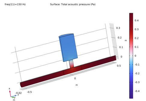
Locate the Data section. From the Dataset list, choose Study 4 - Acoustics, Ma = 0/Solution 5 (sol5).
4
From the Parameter value (freq (Hz)) list, choose 150.
5
Click to expand the Selection section. From the Geometric entity level list, choose Domain.
6
7
Select the Apply to dataset edges check box.
Surface 1
1
Right-click Acoustics: Pressure, Ma = 0 and choose Surface.
2
In the Settings window for Surface, locate the Expression section.
3
In the Expression text field, type acpr.p_t.
4
Locate the Coloring and Style section. Click  Change Color Table.
5
In the Color Table dialog box, select Wave>Wave in the tree.
6
7
In the Settings window for Surface, locate the Coloring and Style section.
8
From the Scale list, choose Linear symmetric.
9
In the Acoustics: Pressure, Ma = 0 toolbar, click  Plot.
The plot should reproduce Figure 5.
Acoustics: Pressure, Ma = 0.1
1
In the Home toolbar, click  Add Plot Group and choose 3D Plot Group.
2
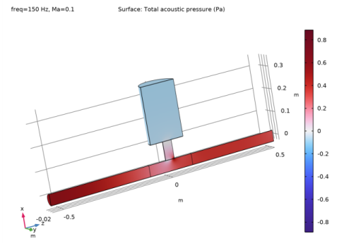
In the Settings window for 3D Plot Group, type Acoustics: Pressure, Ma = 0.1 in the Label text field.
3
Locate the Data section. From the Dataset list, choose Study 3 - Acoustics, Ma = 0.05 and Ma = 0.1/Solution 4 (sol4).
4
From the Parameter value (freq (Hz)) list, choose 150.
5
Locate the Selection section. From the Geometric entity level list, choose Domain.
6
7
Select the Apply to dataset edges check box.
Surface 1
1
Right-click Acoustics: Pressure, Ma = 0.1 and choose Surface.
2
In the Settings window for Surface, locate the Expression section.
3
In the Expression text field, type lnsf.p_t.
4
Locate the Coloring and Style section. Click  Change Color Table.
5
In the Color Table dialog box, select Wave>Wave in the tree.
6
7
In the Settings window for Surface, locate the Coloring and Style section.
8
From the Scale list, choose Linear symmetric.
9
In the Acoustics: Pressure, Ma = 0.1 toolbar, click  Plot.
The plot should reproduce Figure 7.
Change the Flow Mach number to reproduce the results in Figure 6.
Acoustics: Sound Pressure Level, Ma = 0.05
1
Right-click Surface 1 and choose Duplicate.
2
In the Model Builder window, click Acoustics: Pressure, Ma = 0.1.1.
3
In the Settings window for 3D Plot Group, type Acoustics: Sound Pressure Level, Ma = 0.05 in the Label text field.
4
Locate the Data section. From the Parameter value (Ma) list, choose 0.05.
Surface 1
1
In the Model Builder window, click Surface 1.
2
In the Settings window for Surface, locate the Expression section.
3
In the Expression text field, type lnsf.Lp.
4
Locate the Coloring and Style section. Click  Change Color Table.
5
In the Color Table dialog box, select Rainbow>Rainbow in the tree.
6
7
In the Settings window for Surface, locate the Coloring and Style section.
8
From the Scale list, choose Linear.
9
Click to expand the Quality section. From the Resolution list, choose Finer.
10
In the Acoustics: Sound Pressure Level, Ma = 0.05 toolbar, click  Plot.
Transmission Loss
1
In the Home toolbar, click  Add Plot Group and choose 1D Plot Group.
2
In the Settings window for 1D Plot Group, type Transmission Loss in the Label text field.
3
Locate the Data section. From the Dataset list, choose None.
4
Locate the Title section. From the Title type list, choose Label.
5
Locate the Plot Settings section.
6
Select the x-axis label check box. In the associated text field, type f (Hz).
7
Select the y-axis label check box. In the associated text field, type TL (dB).
8
Locate the Axis section. Select the Manual axis limits check box.
9
In the y minimum text field, type 0.
10
In the y maximum text field, type 40.
11
In the x minimum text field, type 50.
12
In the x maximum text field, type 200.
Global 1
1
Right-click Transmission Loss and choose Global.
2
In the Settings window for Global, locate the Data section.
3
From the Dataset list, choose Study 4 - Acoustics, Ma = 0/Solution 5 (sol5).
4
Locate the y-Axis Data section. In the table, enter the following settings:
5
Click to expand the Coloring and Style section. Find the Line markers subsection. From the Marker list, choose Point.
Global 2
1
In the Model Builder window, right-click Transmission Loss and choose Global.
2
In the Settings window for Global, locate the Data section.
3
From the Dataset list, choose Study 3 - Acoustics, Ma = 0.05 and Ma = 0.1/Solution 4 (sol4).
4
Locate the y-Axis Data section. In the table, enter the following settings:
5
Locate the x-Axis Data section. From the Axis source data list, choose freq.
6
Locate the Coloring and Style section. Find the Line markers subsection. From the Marker list, choose Point.
The plot should reproduce Figure 8.
The last thing to do is to disable the PMLs in the CFD study. This is to make sure that, if the study is solved again then the results will be correct. The CFD interface is not supported inside domains with PMLs.
Study 1 - CFD
Step 1: Wall Distance Initialization
1
In the Model Builder window, under Study 1 - CFD click Step 1: Wall Distance Initialization.
2
In the Settings window for Wall Distance Initialization, locate the Physics and Variables Selection section.
3
Select the Modify model configuration for study step check box.
4
In the tree, select Component 1 (comp1)>Definitions>Artificial Domains>Perfectly Matched Layer 1 (pml1).
5
Step 2: Stationary
1
In the Model Builder window, click Step 2: Stationary.
2
In the Settings window for Stationary, locate the Physics and Variables Selection section.
3
Select the Modify model configuration for study step check box.
4
In the tree, select Component 1 (comp1)>Definitions>Artificial Domains>Perfectly Matched Layer 1 (pml1).
5