You are viewing the documentation for an older COMSOL version. The latest version is available here.
PDF

Gaussian Pulse in 2D Uniform Flow:
Convected Wave Equation and Absorbing Layers
Introduction
This small tutorial is a standard test and benchmark model for nonreflecting conditions and sponge layers for linearized Euler like systems, see Ref. 1 and Ref. 2. The Convected Wave Equation, Time Explicit interface solves the linearized Euler equations with an adiabatic equation of state and the interface has the Absorbing Layers to model infinite domains.
An acoustic pulse is generated by an initial Gaussian distribution at the center of the computational domain. The pulse propagates in a high Mach number uniform flow. An analytical solution exists to the problem and is used to validate the solution. The model shows how to set up and use the absorbing layers.
Model Definition
The computational domain with absorbing layers is depicted in Figure 1. The model is set up in a dimensionless system where the speed of sound c= 1 and the density ρ0 = 1. The Gaussian pulse is emitted at the origin x = 0 with initial values
(1)
where α = ln(2)/9 and β = 0.04. The parameters and the expressions for the initial values are defined as parameters and variables and loaded from files during the model setup. The pulse propagates in a uniform background flow u0 = (Ma,0), where Ma = 0.5. The analytical solution to Equation 1 is given by (see Ref. 2)
(2)
In the model, the integrate() operator is used to express the analytical solution. The integration is performed on a finite interval.
Figure 1: Geometry, physical domain and absorbing layers.
Results and Discussion
The propagation of the acoustic pulse is depicted in Figure 2 and Figure 3. The two figures show the acoustic pressure and the acoustic particle velocity, respectively, at four consecutive time instances. In Figure 4, the pressure and velocity are depicted at the final simulated time t = 120. Here, the pulse is inside the absorbing layer. It is evident how the scaling in the layer slows the pulse (it moves slower and slower toward the outer edges) and makes it propagate more normal to the outer boundary. This shows one of the principles of the absorbing layer. The other two mechanisms at work is filtering and a simple impedance condition at the outer boundary.
In the final two figures, the simulated results are compared with the analytical solution. In Figure 5, the pressure at point (20, 30) is depicted as function of time. In Figure 6, the pressure is depicted along the x-axis at t = 50. Both show very good agreement with the analytical solution. The absorbing layers can under optimal condition reduce the spuriously reflected waves to 1/1000 of the incident field amplitude.
Figure 2: The pressure profile at different time steps.
Figure 3: The acoustic velocity profiles at different time steps.
Figure 4: The pressure profile (left) and acoustic velocity profile (right) at the final simulated time t = 120.
Figure 5: The pressure as function of time in point (x,y) = (20,30). The model solution compared with the analytical solution.
Figure 6: Pressure profile along the x-axis at t = 50 comparing the analytical solution and the COMSOL solution.
References
1. H.L. Atkins, “Application of Essentially Nonoscillatory Methods to Aeroacoustic Flow Problems,” Proceedings of ICASE/LaRCWorkshop on Benchmark Problems in Computational Aeroacoustics, edited by J.C. Hardin, J.R. Ristorcelli, and C.K.W. Tam, NASA CP-3300, pp. 15–26, 1995.
2. H.L. Atkins and C.W. Shu, “Quadrature-Free Implementation of Discontinuous Galerkin Method for Hyperbolic Equations,” AIAA Journal, vol. 36, pp. 775–782, 1998.
Application Library path: Acoustics_Module/Tutorials,_Pressure_Acoustics/gaussian_pulse_absorbing_layers
Modeling Instructions
From the File menu, choose New.
New
In the New window, click  Model Wizard.
Model Wizard
1
In the Model Wizard window, click  2D.
2
In the Select Physics tree, select Acoustics>Ultrasound>Convected Wave Equation, Time Explicit (cwe).
3
Click Add.
4
Click  Study.
5
In the Select Study tree, select General Studies>Time Dependent.
6
Global Definitions
Load the parameters used to define the geometry, the Gaussian pulse, and the background flow properties.
Parameters 1
1
In the Model Builder window, under Global Definitions click Parameters 1.
2
In the Settings window for Parameters, locate the Parameters section.
3
Click  Load from File.
4
Geometry 1
Square 1 (sq1)
1
In the Geometry toolbar, click  Square.
2
In the Settings window for Square, locate the Size section.
3
In the Side length text field, type W.
4
Locate the Position section. From the Base list, choose Center.
5
Click to expand the Layers section. Select the Layers to the left check box.
6
Select the Layers to the right check box.
7
Select the Layers on top check box.
8
9
Click  Build All Objects.
The geometry consists of a physical domain surrounded by the absorbing layers, see Figure 1.
Definitions
Next, load the variables that define the initial Gaussian shape (acoustic pressure and velocity components) and then set up the absorbing layers.
Variables 1
1
In the Model Builder window, expand the Component 1 (comp1)>Definitions node.
2
Right-click Definitions and choose Variables.
3
In the Settings window for Variables, locate the Variables section.
4
Click  Load from File.
5
Absorbing Layer 1 (ab1)
1
In the Definitions toolbar, click  Absorbing Layer.
2
Root
Before setting up the physics, change the unit system to be dimensionless.
1
In the Model Builder window, click the root node.
2
In the root node’s Settings window, locate the Unit System section.
3
From the Unit system list, choose None.
Convected Wave Equation, Time Explicit (cwe)
At the physics interface level, there are a number of interesting settings. Some are hidden per default. Start by enabling the Advanced Physics options to be able to see the Filter Parameters for Absorbing Layers section.
1
Click the  Show More Options button in the Model Builder toolbar.
2
In the Show More Options dialog box, in the tree, select the check box for the node Physics>Advanced Physics Options.
3
In the same way, you can also access the Discretization section by enabling it. Notice that the default discretization for both the pressure and the velocity is Quartic, that is, fourth order. Further details about this choice and the time explicit method used in the Convected Wave Equation interface can be found in the Acoustics Module User’s Guide.
Convected Wave Equation Model 1
1
In the Model Builder window, under Component 1 (comp1)>Convected Wave Equation, Time Explicit (cwe) click Convected Wave Equation Model 1.
2
In the Settings window for Convected Wave Equation Model, locate the Model Input section.
3
In the p0 text field, type p0.
4
Specify the u0 vector as
5
Locate the Fluid Properties section. From the ρ0 list, choose User defined. In the associated text field, type rho0.
6
From the c0 list, choose User defined. In the associated text field, type c0.
Initial Values 1
1
In the Model Builder window, click Initial Values 1.
2
In the Settings window for Initial Values, locate the Initial Values section.
3
In the p text field, type p_i.
4
Specify the u vector as
Finally, set up the impedance condition and apply it on all the outer boundaries. This simple nonreflecting condition is the final piece (combined with filtering and coordinate stretching) that makes the absorbing layers work.
Specific Acoustic Impedance (Isentropic) 1
1
In the Physics toolbar, click  Boundaries and choose Specific Acoustic Impedance (Isentropic).
2
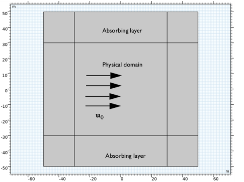
In the Settings window for Specific Acoustic Impedance (Isentropic), locate the Boundary Selection section.
3
From the Selection list, choose All boundaries.
Mesh 1
1
In the Model Builder window, under Component 1 (comp1) click Mesh 1.
2
In the Settings window for Mesh, locate the Physics-Controlled Mesh section.
3
From the Element size list, choose Finer.
For the mesh, we have selected the default Finer setting. A more thorough approach would be to define the mesh size according to the highest frequency component in the model (the smallest wavelength to resolve). For the time explicit discontinuous Galerkin method (with default fourth order discretization), use two mesh elements per wavelength. Guidelines for meshing can be found in the documentation for the interface.
Study 1
Step 1: Time Dependent
Solve the model from time t = 0 to 120 in steps of 1 (dimensionless time units). Simply modify the default expression.
1
In the Model Builder window, under Study 1 click Step 1: Time Dependent.
2
In the Settings window for Time Dependent, locate the Study Settings section.
3
In the Output times text field, type range(0,1,120).
4
In the Home toolbar, click  Compute.
Results
Acoustic Pressure (cwe)
The first default plot shows the acoustic pressure in the computational domain. You can change the times to plot the distribution at various times, see Figure 2 and Figure 4.
1
In the Settings window for 2D Plot Group, locate the Data section.
2
From the Time (s) list, choose 0.
3
In the Acoustic Pressure (cwe) toolbar, click  Plot.
The second default plot shows the acoustic velocity. The plots, for selected times, can be seen in Figure 3 and Figure 4.
Acoustic Velocity (cwe)
1
In the Model Builder window, click Acoustic Velocity (cwe).
2
In the Settings window for 2D Plot Group, locate the Data section.
3
From the Time (s) list, choose 0.
4
In the Acoustic Velocity (cwe) toolbar, click  Plot.
Create some extra datasets to use in the following plots. Create a cut point to plot the pressure as function of time in a desired coordinate set. Create a cut line to plot the pressure along a line for a given time. Finally, create a dataset with a selection restricting the solution to the physical domain (not the absorbing layers).
Cut Point 2D 1
1
In the Results toolbar, click  Cut Point 2D.
2
In the Settings window for Cut Point 2D, locate the Point Data section.
3
In the x text field, type 20.
4
In the y text field, type 10.
Cut Line 2D 1
1
In the Results toolbar, click  Cut Line 2D.
2
In the Settings window for Cut Line 2D, locate the Line Data section.
3
In row Point 1, set x to -50.
4
In row Point 2, set x to 50.
Cut Line 2D 2
1
In the Results toolbar, click  Cut Line 2D.
2
In the Settings window for Cut Line 2D, locate the Line Data section.
3
In row Point 1, set x to -30.
4
In row Point 2, set x to 30.
The pressure as function of time is depicted in Figure 5 where it is compared with the analytical solution.
Pressure in Point
1
In the Results toolbar, click  1D Plot Group.
2
In the Settings window for 1D Plot Group, type Pressure in Point in the Label text field.
3
Locate the Data section. From the Dataset list, choose Cut Point 2D 1.
Point Graph 1
1
Right-click Pressure in Point and choose Point Graph.
2
In the Settings window for Point Graph, click to expand the Legends section.
3
Select the Show legends check box.
4
From the Legends list, choose Manual.
5
Point Graph 2
1
In the Model Builder window, right-click Pressure in Point and choose Point Graph.
2
In the Settings window for Point Graph, locate the y-Axis Data section.
3
In the Expression text field, type p_a.
4
Locate the Legends section. Select the Show legends check box.
5
From the Legends list, choose Manual.
6
7
Click to expand the Coloring and Style section. Find the Line style subsection. From the Line list, choose None.
8
Find the Line markers subsection. From the Marker list, choose Point.
9
From the Positioning list, choose Interpolated.
10
In the Number text field, type 100.
11
In the Pressure in Point toolbar, click  Plot.
The pressure on the x-axis for a given time is depicted in Figure 6 where it is compared with the analytical solution.
Pressure over Cut Line
1
In the Home toolbar, click  Add Plot Group and choose 1D Plot Group.
2
In the Settings window for 1D Plot Group, type Pressure over Cut Line in the Label text field.
3
Locate the Data section. From the Dataset list, choose None.
Line Graph 1
1
Right-click Pressure over Cut Line and choose Line Graph.
2
In the Settings window for Line Graph, locate the Data section.
3
From the Dataset list, choose Cut Line 2D 1.
4
From the Time selection list, choose From list.
5
In the Times (s) list, select 40.
6
Locate the y-Axis Data section. In the Expression text field, type p.
7
Locate the x-Axis Data section. From the Parameter list, choose Expression.
8
In the Expression text field, type x.
9
Click to expand the Legends section. Select the Show legends check box.
10
From the Legends list, choose Manual.
11
12
Click to expand the Quality section. From the Resolution list, choose Extra fine.
13
In the Pressure over Cut Line toolbar, click  Plot.
Line Graph 2
1
In the Model Builder window, right-click Pressure over Cut Line and choose Line Graph.
2
In the Settings window for Line Graph, locate the Data section.
3
From the Dataset list, choose Cut Line 2D 2.
4
From the Time selection list, choose From list.
5
In the Times (s) list, select 40.
6
Locate the y-Axis Data section. In the Expression text field, type p_a.
7
Locate the x-Axis Data section. From the Parameter list, choose Expression.
8
In the Expression text field, type x.
9
Click to expand the Coloring and Style section. Find the Line style subsection. From the Line list, choose None.
10
Find the Line markers subsection. From the Marker list, choose Point.
11
From the Positioning list, choose Interpolated.
12
In the Number text field, type 100.
13
Locate the Legends section. Select the Show legends check box.
14
From the Legends list, choose Manual.
15
16
Locate the Quality section. From the Resolution list, choose Extra fine.
Note that when plotting the solution of the simulation, as function of spatial variables (line plot or a surface), you need to increase the resolution. This is because of the default quartic elements used. The default plots generated already have a higher default resolution.
17
In the Pressure over Cut Line toolbar, click  Plot.
Finally, plot the pressure only in the physical domain. This plot can, for example, be used to create a nice animation. Under the Export > node select Animation and then select the last plot.
Another interesting observation is that the remaining (spuriously) reflected waves have an amplitude which is a factor 1000 smaller than the original signal (from the solution at time t = 0).
Acoustic Pressure (cwe) Selection
1
In the Model Builder window, right-click Acoustic Pressure (cwe) and choose Duplicate.
2
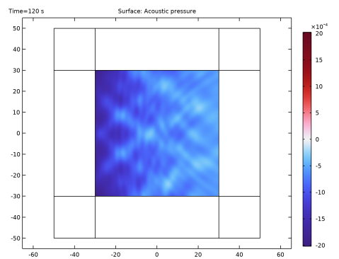
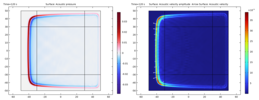
In the Settings window for 2D Plot Group, type Acoustic Pressure (cwe) Selection in the Label text field.
Selection 1
1
In the Model Builder window, expand the Acoustic Pressure (cwe) Selection node.
2
Right-click Acoustic Pressure and choose Selection.
3
4
Click the  Zoom Extents button in the Graphics toolbar.
5
In the Acoustic Pressure (cwe) Selection toolbar, click  Plot.