|
|
|
|
•
|
Using the Electric Currents interface: Current Conservation, Terminal, Ground... Extracting lumped quantities using the terminal feature.
|
|
•
|
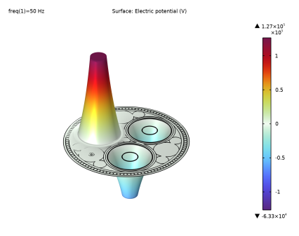
Comparing a numerical model to an analytical one. Comparing displacement- and conduction currents. Checking the risk of electromagnetic breakdown. Checking the conditions on the floating end of a 10 km long cable with single-point bonding applied.
|
|
•
|
Using expressions such as exp(-120[deg]*j) to set a phase difference in the frequency domain. Reflecting on the applicability of the used partial differential equations (whether it is safe to assume the in-plane electric fields are curl-free).
|
|
•
|
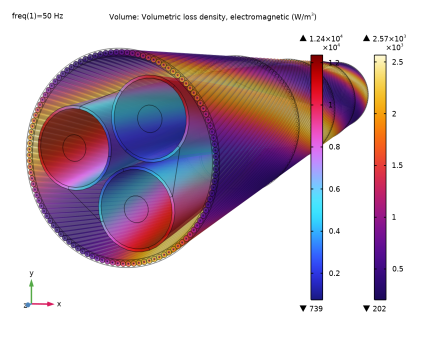
Using the Electric Currents interface: Current Conservation, Electric Potential, Ground... Determining the total loss in a system by means of a volume integration.
|
|
•
|
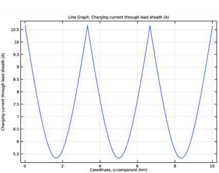
Discussing several bonding types: single-point bonding, solid bonding, and cross bonding, and reflecting on how they affect the build up of charging currents. Comparing a numerical model to analytical ones (one for each bonding type).
|
|
•
|
Using the Magnetic Fields interface: Ampère’s Law, Coil (group), Magnetic Insulation... Exciting a 2D/2.5D inductive model by means of the Coil feature.
|
|
•
|
Using a Coil group to model the armor twist (useful for cross bonding too). Using the Homogenized multiturn setting to approximate a milliken conductor.
|
|
•
|
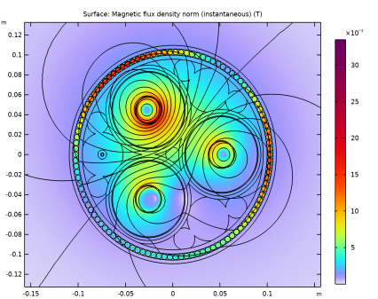
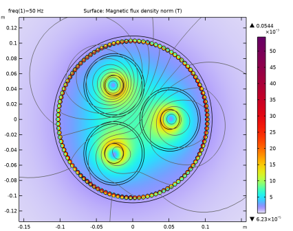
Advanced postprocessing. Analyzing and verifying results, investigating the differences between the Plain 2D, 2.5D and 2.5D + milliken configurations. Reflecting on the difference between the AC- and DC resistance.
|
|
•
|
Using the Magnetic Fields interface: Ampère’s Law, Coil, Magnetic Insulation... Connecting three finite element models in series, using an Electrical Circuit.
|
|
•
|
Discussing several bonding types: single-point bonding, solid bonding, and cross bonding, and reflecting on how they affect the potential and currents in the screens.
|
|
•
|
Validating if cross bonding can be modeled in 2D by means of a Coil group. Comparing the losses and lumped parameters to the detailed plain 2D model from the Inductive Effects tutorial and reflecting on what details are really important.
|
|
•
|
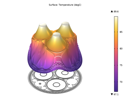
Using the Magnetic Fields interface, the Heat Transfer in Solids interface and the Electromagnetic Heating multiphysics coupling to model induction heating.
|
|
•
|
Using linearized resistivity. Investigating resistive- and magnetic losses. Reflecting on the difference between current-driven and voltage-driven conductors, and how the heat affects the electromagnetic properties of the cable. Investigating the difference between the AC- and DC resistance, and the validity of stationary-electric reasoning.
|
|
•
|
Using a global ODE to set a phase conductivity such that the cable's AC resistance matches a certain specified (temperature dependent) value.
|
|
•
|
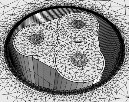
Using advanced geometry handling and meshing to optimize a 3D mesh to produce a high level of detail, while keeping the number of degrees of freedom (DOFs) low.
|
|
•
|
Using highly anisotropic meshes. Combining Swept meshes, Free Tetrahedral meshes, and Boundary Layer meshes. Reflecting on the importance of conforming meshes for periodicity planes. Demonstrating how mesh conformity can be enforced and checked.
|
|
•
|
Using the Magnetic Fields interface in 3D: Ampère’s Law, Coil, twisted Periodicity... Exiting a 3D inductive model by means of a Coil feature (with slanted cut), combined with a Coil Geometry Analysis preprocessing step.
|
|
•
|
A demonstration of twisted periodicity and short-twisted periodicity, phase- and armor lay length, first- (and higher) order temperature corrections, and the analysis of resistive and magnetic losses in the phases, the screens, and the armor.
|
|
•
|
A detailed comparison between the 3D twist models — with or without linearized resistivity included — and 2D/2.5D models (with or without induction heating).
|
|
•
|
A reflection on numerical stability and the demonstration of a numerical stabilization method that manages to improve the accuracy while keeping the solving time low.
|
|
1
|
|
2
|
Click
|
|
1
|
|
2
|
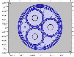
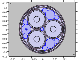
Browse to the model’s Application Libraries folder and double-click the file submarine_cable_e_geom_sequence.mph.
|
|
3
|
|
4
|
|
1
|
|
2
|
|
1
|
|
2
|
|
3
|
|
4
|
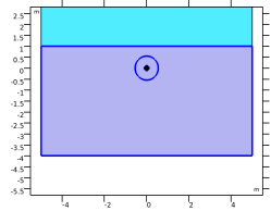
Browse to the model’s Application Libraries folder and double-click the file submarine_cable_b_geom_parameters.txt.
|
|
1
|
|
2
|
|
3
|
|
4
|
|
5
|
Click OK.
|
|
6
|
|
1
|
|
2
|
|
3
|
|
4
|
In the Add dialog box, in the Selections to add list, choose Phases, Screens, Steel Helix (Fiber), and Cable Armor.
|
|
5
|
Click OK.
|
|
6
|
|
1
|
|
2
|
|
3
|
|
4
|
|
5
|
Click OK.
|
|
6
|
|
7
|
|
8
|
In the Add dialog box, in the Selections to subtract list, choose Metals, Semiconductive Compound, and Cross-Linked Polyethylene (XLPE).
|
|
9
|
Click OK.
|
|
10
|
|
1
|
|
2
|
|
3
|
|
4
|
|
5
|
Click OK.
|
|
6
|
|
7
|
|
1
|
|
2
|
|
3
|
|
1
|
|
2
|
|
3
|
In the tree, select Built-in>Air.
|
|
4
|
|
5
|
|
6
|
|
1
|
|
1
|
|
3
|
|
1
|
|
2
|
|
4
|
|
5
|
Locate the Material Properties section. In the Material properties tree, select Basic Properties>Relative Permeability.
|
|
6
|
|
7
|
Repeat these steps for Electrical Conductivity, Relative Permittivity, Thermal Conductivity, Density, and Heat Capacity at Constant Pressure.
|
|
8
|
Click to collapse the Material Properties section. Click to expand the Appearance section. From the Material type list, choose Rock.
|
|
1
|
|
2
|
|
3
|
|
4
|
|
5
|
|
1
|
|
2
|
|
3
|
|
4
|
|
5
|
|
1
|
|
2
|
|
3
|
Locate the Geometric Entity Selection section. From the Selection list, choose Cross-Linked Polyethylene (XLPE).
 |
|
4
|
|
1
|
|
2
|
|
3
|
Locate the Geometric Entity Selection section. From the Selection list, choose Semiconductive Compound.
 |
|
4
|
|
1
|
|
2
|
|
3
|
|
1
|
|
2
|
|
3
|
|
1
|
|
2
|
|
3
|
|
4
|
|
1
|
In the Model Builder window, under Component 1 (comp1)>Materials right-click Bitumen compound (mat8) and choose Duplicate (make sure to duplicate the bitumen, not the glass).
|
|
2
|
|
3
|
|
4
|
|
1
|
|
2
|
|
3
|
|
4
|
|
5
|
Locate the Material Properties section. In the Material properties tree, select Electromagnetic Models>Linearized Resistivity.
|
|
6
|
|
7
|
Click to collapse the Material Properties section. Click to expand the Appearance section. From the Material type list, choose Copper.
|
|
1
|
|
2
|
|
3
|
|
4
|
|
5
|
|
1
|
|
2
|
|
3
|
|
4
|
|
5
|
|
6
|
|
7
|
In the Model Builder window, under Component 1 (comp1)>Materials, check whether the following materials are present:
|
|
1
|
In the Model Builder window, under Component 1 (comp1)>Materials, add the following material properties:
|
|
1
|
|
1
|
|
2
|
Browse to a suitable folder and type the filename submarine_cable_01_introduction.mph.
|
|
1
|
|
2
|
|
3
|
|
4
|
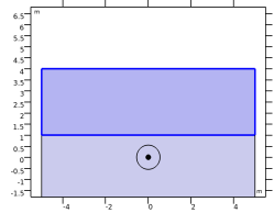
Browse to the model’s Application Libraries folder and double-click the file submarine_cable_a_geom_parameters.txt.
|
|
1
|
|
2
|
|
3
|
|
4
|
|
5
|
|
6
|
|
7
|
Locate the Selections of Resulting Entities section. Select the Resulting objects selection check box.
|
|
8
|
|
9
|
|
1
|
|
2
|
|
3
|
|
4
|
|
5
|
Locate the Selections of Resulting Entities section. Select the Resulting objects selection check box.
|
|
6
|
|
7
|
|
1
|
|
2
|
|
3
|
|
4
|
|
5
|
|
6
|
|
7
|
Locate the Selections of Resulting Entities section. Select the Resulting objects selection check box.
|
|
8
|
|
9
|
|
1
|
|
2
|
|
3
|
|
4
|
|
5
|
|
6
|
Click to expand the Layers section. In the table, enter the following settings:
|
|
7
|
|
1
|
|
2
|
|
3
|
|
4
|
|
5
|
|
6
|
Locate the Layers section. In the table, enter the following settings:
|
|
7
|
|
8
|
|
1
|
|
2
|
|
3
|
|
4
|
|
5
|
|
6
|
Locate the Layers section. In the table, enter the following settings:
|
|
7
|
|
1
|
|
2
|
|
3
|
|
4
|
|
5
|
|
6
|
Locate the Layers section. In the table, enter the following settings:
|
|
7
|
|
1
|
|
2
|
|
3
|
|
4
|
|
5
|
Locate the Selections of Resulting Entities section. Select the Resulting objects selection check box.
|
|
6
|
|
1
|
|
2
|
|
3
|
|
4
|
|
5
|
Locate the Selections of Resulting Entities section. Select the Resulting objects selection check box.
|
|
6
|
|
1
|
|
2
|
|
3
|
|
4
|
|
5
|
Locate the Selections of Resulting Entities section. Select the Resulting objects selection check box.
|
|
6
|
|
1
|
|
2
|
|
3
|
|
4
|
|
5
|
|
6
|
Locate the Layers section. In the table, enter the following settings:
|
|
7
|
|
1
|
|
2
|
|
3
|
|
4
|
|
5
|
|
6
|
|
7
|
|
1
|
|
2
|
|
3
|
|
4
|
|
5
|
|
6
|
|
1
|
|
2
|
|
3
|
|
4
|
|
5
|
Locate the Layers section. In the table, enter the following settings:
|
|
6
|
|
7
|
|
1
|
|
2
|
|
3
|
|
4
|
|
5
|
Locate the Layers section. In the table, enter the following settings:
|
|
6
|
|
1
|
|
2
|
|
3
|
|
4
|
Locate the Difference section. Find the Objects to subtract subsection. Click to select the
|
|
5
|
|
6
|
|
7
|
Locate the Selections of Resulting Entities section. Select the Resulting objects selection check box.
|
|
8
|
|
1
|
|
2
|
|
3
|
|
4
|
|
5
|
|
1
|
|
2
|
|
3
|
|
4
|
|
5
|
|
6
|
|
1
|
|
2
|
|
3
|
|
4
|
|
1
|
|
2
|
|
3
|
|
4
|
|
5
|
Locate the Selections of Resulting Entities section. Select the Resulting objects selection check box.
|
|
6
|
|
7
|
|
1
|
|
2
|
|
3
|
|
4
|
|
1
|
|
2
|
|
3
|
|
4
|
|
5
|
|
1
|
|
2
|
|
3
|
|
4
|
Locate the Selections of Resulting Entities section. Select the Resulting objects selection check box.
|
|
5
|
|
6
|
|
1
|
|
2
|
|
3
|
|
4
|
|
5
|
|
6
|
|
7
|
|
8
|
|
9
|
Locate the Selections of Resulting Entities section. Select the Resulting objects selection check box.
|
|
10
|
|
1
|
|
2
|
|
3
|
|
4
|
|
5
|
|
6
|
|
1
|
|
2
|
|
3
|
|
4
|
|
5
|
|
6
|
Locate the Layers section. In the table, enter the following settings:
|
|
7
|
Locate the Selections of Resulting Entities section. Select the Resulting objects selection check box.
|
|
8
|
|
1
|
|
2
|
|
3
|
|
4
|
|
5
|
Locate the Selections of Resulting Entities section. Select the Resulting objects selection check box.
|
|
6
|
|
1
|
|
2
|
|
3
|
|
4
|
|
5
|
Locate the Selections of Resulting Entities section. Select the Resulting objects selection check box.
|
|
6
|
|
1
|
|
2
|
|
3
|
|
4
|
|
5
|
|
6
|
|
1
|
In the Model Builder window, under Component 1 (comp1)>Geometry 1 right-click Circle 10 (c10) and choose Duplicate.
|
|
2
|
|
3
|
|
4
|
|
5
|
|
1
|
|
2
|
|
3
|
|
4
|
Locate the Selections of Resulting Entities section. Select the Resulting objects selection check box.
|
|
5
|
|
6
|
|
1
|
|
2
|
|
3
|
|
4
|
|
5
|
|
6
|
|
7
|
Locate the Selections of Resulting Entities section. Select the Resulting objects selection check box.
|
|
8
|
|
1
|
|
2
|
|
3
|
|
4
|
Locate the Selections of Resulting Entities section. Select the Resulting objects selection check box.
|
|
5
|
|
1
|
|
2
|
|
3
|
|
4
|
Locate the Selections of Resulting Entities section. Select the Resulting objects selection check box.
|
|
5
|
|
6
|
|
1
|
|
2
|
|
3
|
|
4
|
|
5
|
|
6
|
|
7
|
Click to expand the Layers section. In the table, enter the following settings:
|
|
8
|
Locate the Selections of Resulting Entities section. Select the Resulting objects selection check box.
|
|
9
|
|
10
|
|
1
|
In the Model Builder window, under Component 1 (comp1) right-click Materials and choose Blank Material.
|
|
2
|
|
3
|
|
4
|
|
5
|
|
6
|
|
7
|
|
8
|
|
9
|
|
10
|
|
11
|
|
12
|
|
13
|
|
14
|
|
15
|
|
16
|
|
17
|
|
18
|
|
19
|
|
20
|
|
21
|