PDF

Electric Field from Power Lines
Introduction
Power lines are commonly used as a means of transmitting electrical power across large distances. In this tutorial, two towers transmitting high voltage three-phase AC power are modeled, and the resulting electric field is computed. Specifically, the voltage is set to 400 kV in this model. In transmission lines with such a high voltage, the phase lines are usually made up of several smaller conductors bundled together. For simplicity, a single conductor for each phase line is used in this model, but its radius is set to 10 cm in order to simulate the effective radius of a bundled conductor.
The towers also have two shielding lines above the phase lines, which protect the tower from lightning strikes. These shielding lines have a slightly smaller radius, which in this model is set to 1 cm.
Model Definition
The geometry of one of the towers is shown in Figure 1. It is imported from an external file due to its complexity. The ground level in this geometry is created using a geometry part from the Part Library, which creates a flat surface that is randomly perturbed. Note that the insulators purely are for aesthetic purposes in this model.
Figure 1: The geometry of the transmission tower. The two shielding lines can be seen on top, while the three phase lines are held by the insulators.
To solve the model, use the 3D Electrostatics, Boundary Elements interface in the AC/DC Module. In this physics interface, the electric scalar potential, V, satisfies the equation
where ε0 is the permittivity of free space, εr is the relative permittivity, and ρ is the space charge density. The electric field and the displacement field are derived from the potential:
In the model, the Ground feature sets the boundary condition V = 0 at the shielding lines, the tower, and the floor. On the phase lines, the Electric Potential feature is used to set the specified potentials, each of them phase shifted with respect to the others. Since the wires are edges in the geometry, it is also necessary to specify the corresponding edge radius for each such feature.
Since the model is using the boundary element method (BEM), and the potential is fixed at all the edges and surfaces, it only needs to solve the above equations in the infinite void surrounding the towers. This also illustrates the strength of using BEM in models where there are large empty spaces. If it instead had used the finite element method (FEM), like most other physics interfaces, it would have needed to create a volumetric mesh in the entire air domain. This would have significantly increased the number of degrees of freedom, which is likely to also increase the time required to solve the model.
Results
The electric field norm from the wires at ground level is shown Figure 2, along with streamlines showing the direction of the electric field,
Figure 2: The electric field norm (surface) and the electric field (streamlines) from the transmission lines.
Application Library path: ACDC_Module/Devices,_Capacitive/power_line_electric_field
Modeling Instructions
From the File menu, choose New.
New
In the New window, click  Model Wizard.
Model Wizard
1
In the Model Wizard window, click  3D.
2
In the Select Physics tree, select AC/DC>Electric Fields and Currents>Electrostatics, Boundary Elements (esbe).
3
Click Add.
4
Click  Study.
5
In the Select Study tree, select General Studies>Frequency Domain.
6
First, define some parameters that will be used when building the model.
Global Definitions
Parameters 1
1
In the Model Builder window, under Global Definitions click Parameters 1.
2
In the Settings window for Parameters, locate the Parameters section.
3
For the sake of simplicity, the geometry of the model will be imported from an external file. Note that since the boundary element method is used in this model, there is no need for an air domain in the geometry.
Geometry 1
Import 1 (imp1)
1
In the Home toolbar, click  Import.
2
In the Settings window for Import, locate the Import section.
3
Click  Browse.
4
5
Click  Import.
Add Material
1
In the Home toolbar, click  Add Material to open the Add Material window.
2
Go to the Add Material window.
3
4
Click Add to Component in the window toolbar.
5
In the Home toolbar, click  Add Material to close the Add Material window.
Materials
Air (mat1)
1
In the Settings window for Material, locate the Geometric Entity Selection section.
2
From the Geometric entity level list, choose Domain.
3
From the Selection list, choose All voids.
In the physics interface, add phase shifted electric potentials on the three phase lines. Also, add ground at the towers, the shielding lines, and the floor.
Electrostatics, Boundary Elements (esbe)
Electric Potential 1
1
In the Model Builder window, under Component 1 (comp1) right-click Electrostatics, Boundary Elements (esbe) and choose Edges>Electric Potential.
2
In the Settings window for Electric Potential, locate the Electric Potential section.
3
In the V0 text field, type V0.
4
Locate the Edge Radius section. In the Edge radius text field, type r0.
5
Locate the Edge Selection section. Click  Paste Selection.
6
In the Paste Selection dialog box, type 66, 75, 94 in the Selection text field.
7
Electric Potential 2
1
In the Physics toolbar, click  Edges and choose Electric Potential.
2
In the Settings window for Electric Potential, locate the Electric Potential section.
3
In the V0 text field, type V0*exp(i*2*pi/3).
4
Locate the Edge Radius section. In the Edge radius text field, type r0.
5
Locate the Edge Selection section. Click  Paste Selection.
6
In the Paste Selection dialog box, type 802, 820, 856 in the Selection text field.
7
Electric Potential 3
1
In the Physics toolbar, click  Edges and choose Electric Potential.
2
In the Settings window for Electric Potential, locate the Electric Potential section.
3
In the V0 text field, type V0*exp(i*4*pi/3).
4
Locate the Edge Radius section. In the Edge radius text field, type r0.
5
Locate the Edge Selection section. Click  Paste Selection.
6
In the Paste Selection dialog box, type 1550, 1559, 1578 in the Selection text field.
7
Ground 1
1
In the Physics toolbar, click  Boundaries and choose Ground.
2
In the Settings window for Ground, locate the Boundary Selection section.
3
Click  Paste Selection.
4
In the Paste Selection dialog box, type 1 in the Selection text field.
5
Ground 2
1
In the Physics toolbar, click  Edges and choose Ground.
2
In the Settings window for Ground, locate the Edge Radius section.
3
In the Edge radius text field, type rs.
4
Locate the Edge Selection section. Click  Paste Selection.
5
In the Paste Selection dialog box, type 467, 484, 508, 1239, 1255, 1278 in the Selection text field.
6
Ground 3
1
In the Physics toolbar, click  Edges and choose Ground.
2
In the Settings window for Ground, locate the Edge Selection section.
3
Click  Paste Selection.
4
In the Paste Selection dialog box, type 4-21, 36, 37, 52-65, 74, 76, 77, 85, 93, 95, 96, 104-466, 468-483, 485-507, 509-769, 784, 785, 800, 801, 803-810, 818, 819, 821, 822, 830-846, 854, 855, 857, 858, 866-1238, 1240-1254, 1256-1277, 1279-1509, 1524, 1525, 1540-1549, 1558, 1560, 1561, 1569, 1577, 1579, 1580, 1588-1602 in the Selection text field.
5
Before solving, refine the mesh. This makes the resulting plots more detailed, and since there is no volumetric mesh in the model, it does not have as large of an impact on solving time as when using FEM.
Mesh 1
1
In the Model Builder window, under Component 1 (comp1) click Mesh 1.
2
In the Settings window for Mesh, locate the Physics-Controlled Mesh section.
3
From the Element size list, choose Extra fine.
4
Click  Build All.
Study 1
Step 1: Frequency Domain
1
In the Model Builder window, under Study 1 click Step 1: Frequency Domain.
2
In the Settings window for Frequency Domain, locate the Study Settings section.
3
In the Frequencies text field, type 50.
4
In the Model Builder window, click Study 1.
5
In the Settings window for Study, locate the Study Settings section.
6
Clear the Generate default plots check box.
7
In the Home toolbar, click  Compute.
Results
In the Model Builder window, expand the Results node.
Grid 3D 1
1
In the Model Builder window, expand the Results>Datasets node.
2
Right-click Results>Datasets and choose More 3D Datasets>Grid 3D.
3
In the Settings window for Grid 3D, locate the Parameter Bounds section.
4
Find the First parameter subsection. In the Minimum text field, type -150.
5
In the Maximum text field, type 150.
6
Find the Second parameter subsection. In the Minimum text field, type -150.
7
In the Maximum text field, type 150.
8
Find the Third parameter subsection. In the Maximum text field, type 100.
Electric Field Norm (surface)
1
In the Results toolbar, click  3D Plot Group.
2
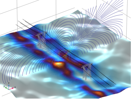
In the Settings window for 3D Plot Group, type Electric Field Norm (surface) in the Label text field.
3
Locate the Data section. From the Dataset list, choose Grid 3D 1.
4
Click to expand the Title section. From the Title type list, choose None.
5
Locate the Color Legend section. Clear the Show legends check box.
6
Locate the Plot Settings section. Clear the Plot dataset edges check box.
Line 1
1
Right-click Electric Field Norm (surface) and choose Line.
2
In the Settings window for Line, locate the Data section.
3
From the Dataset list, choose Study 1/Solution 1 (sol1).
4
Locate the Expression section. In the Expression text field, type 1.
5
Locate the Coloring and Style section. From the Line type list, choose Tube.
6
In the Tube radius expression text field, type 0.1.
7
Select the Radius scale factor check box.
8
From the Coloring list, choose Uniform.
9
From the Color list, choose Black.
Selection 1
1
Right-click Line 1 and choose Selection.
2
In the Settings window for Selection, locate the Selection section.
3
Click  Paste Selection.
4
In the Paste Selection dialog box, type 4-21, 55, 56, 59, 60, 62-65, 76, 77, 95, 96, 106, 108, 110, 112-466, 468-483, 485-507, 509-769, 803-810, 818, 821, 822, 830, 832-846, 854, 857, 858, 866, 868-1238, 1240-1254, 1256-1277, 1279-1509, 1543, 1544, 1547, 1548, 1560, 1561, 1579, 1580, 1589-1592, 1594, 1596, 1598, 1600-1602 in the Selection text field.
5
Material Appearance 1
1
In the Model Builder window, right-click Line 1 and choose Material Appearance.
2
In the Settings window for Material Appearance, locate the Appearance section.
3
From the Appearance list, choose Custom.
4
From the Material type list, choose Steel.
Line 2
1
In the Model Builder window, right-click Electric Field Norm (surface) and choose Line.
2
In the Settings window for Line, locate the Data section.
3
From the Dataset list, choose Study 1/Solution 1 (sol1).
4
Locate the Expression section. In the Expression text field, type 1.
5
Locate the Coloring and Style section. From the Line type list, choose Tube.
6
In the Tube radius expression text field, type 0.1.
7
Select the Radius scale factor check box.
8
From the Coloring list, choose Uniform.
9
From the Color list, choose Black.
Selection 1
1
Right-click Line 2 and choose Selection.
2
In the Settings window for Selection, locate the Selection section.
3
Click  Paste Selection.
4
In the Paste Selection dialog box, type 22-54, 57, 58, 61, 67-74, 78-93, 97-105, 107, 109, 111, 770-801, 811-817, 819, 823-829, 831, 847-853, 855, 859-865, 867, 1510-1542, 1545, 1546, 1549, 1551-1558, 1562-1577, 1581-1588, 1593, 1595, 1597, 1599 in the Selection text field.
5
Line 3
1
In the Model Builder window, right-click Electric Field Norm (surface) and choose Line.
2
In the Settings window for Line, locate the Data section.
3
From the Dataset list, choose Study 1/Solution 1 (sol1).
4
Locate the Expression section. In the Expression text field, type 1.
5
Locate the Coloring and Style section. From the Coloring list, choose Uniform.
6
From the Color list, choose Black.
Selection 1
1
Right-click Line 3 and choose Selection.
2
In the Settings window for Selection, locate the Selection section.
3
Click  Paste Selection.
4
In the Paste Selection dialog box, type 66, 75, 94, 802, 820, 856, 1550, 1559, 1578, 467, 484, 508, 1239, 1255, 1278 in the Selection text field.
5
Surface 1
1
In the Model Builder window, right-click Electric Field Norm (surface) and choose Surface.
2
In the Settings window for Surface, locate the Data section.
3
From the Dataset list, choose Study 1/Solution 1 (sol1).
4
Locate the Expression section. In the Expression text field, type esbe.normE.
5
Locate the Coloring and Style section. Click  Change Color Table.
6
In the Color Table dialog box, select Thermal>ThermalWave in the tree.
7
Selection 1
1
Right-click Surface 1 and choose Selection.
2
In the Settings window for Selection, locate the Selection section.
3
Click  Paste Selection.
4
In the Paste Selection dialog box, type 1 in the Selection text field.
5
Electric Field Norm (surface)
In the Model Builder window, under Results click Electric Field Norm (surface).
Streamline Multislice 1
1
In the Electric Field Norm (surface) toolbar, click  More Plots and choose Streamline Multislice.
2
In the Settings window for Streamline Multislice, locate the Multiplane Data section.
3
Find the x-planes subsection. In the Planes text field, type 0.
4
Find the z-planes subsection. In the Planes text field, type 0.
5
Locate the Streamline Positioning section. From the Positioning list, choose Uniform density.
6
In the Separating distance text field, type 0.02.
Color Expression 1
1
Right-click Streamline Multislice 1 and choose Color Expression.
2
In the Settings window for Color Expression, locate the Expression section.
3
In the Expression text field, type esbe.normE.
Electric Field Norm (surface)
1
In the Model Builder window, under Results click Electric Field Norm (surface).
2
In the Electric Field Norm (surface) toolbar, click  Plot.