PDF

Permanent Magnet Motor in 2D
Introduction
This tutorial model shows how to set up a three-phase permanent magnet motor simulation in 2D, using motor parts that are available in the AC/DC Module Part Library. The model consists of three studies. First, a stationary study solves the problem with a direct current, through the angular span of one pole pair, using Arkkio’s method to calculate the rotor torque. Then, by specifying the initial mechanical angle to yield maximum torque, a transient study solves the time-dependent problem for a complete electrical period, and calculates the results for torque ripple and radial magnetic flux density. Finally, using the results from the transient study, the loss density in the stator iron is calculated with a frequency domain study.
Modeling
This model is set up in 2D and simulates the cross section on the rotational axis of the PM motor. The relevant equation is
where A is the magnetic vector potential which defines the magnetic flux density ∇ × A, J is the current density, and μ is the magnetic permeability. The equation is solved for the out-of-plane vector component only, which implies that in-plane currents and out-of-plane magnetic fields are neglected. This is a justified assumption for the 2D model which greatly simplifies and stabilizes the problem.
The separate rotor and stator objects are built as an assembly, and the relative rotation between rotor and stator is handled by the Rotating Domain node of the Moving Mesh feature, which includes all effects of relative motion between the parts. The domains are connected in the physics via boundary conditions on the continuity pair boundary, which resides in the air gap between them. This continuity pair allows for mesh discontinuities across the boundary where variables can be interpolated between the two independent meshes, ensuring continuity in the magnetic vector potential.
The torque is computed with the Arkkio Torque Calculation feature, which is automatically applied on the air gap domain adjacent to the continuity pair. The losses in the rotor and stator iron are calculated using a Loss Calculation subnode and a Time to Frequency Losses study. In the coils, the losses are Ohmic, while the losses in the iron are computed with the Steinmetz loss model.
Results and Discussion
The objective of the first study is to find the initial mechanical angle which produces the maximum torque on the rotor. As seen in Figure 1, the parametric sweep of the initial angle yields a curve displaying two extremes: one corresponding to accelerating torque, and the other corresponding to deceleration in the direction of the prescribed counter-clockwise rotation. For the maximum accelerating torque, the former is chosen for the initial angle. The subsequent transient study solves the synchronous rotation of the stator field and the rotor. Figure 2 plots the rotor torque ripple as a function of time for one electrical period. Finally, a Time to Frequency Losses study calculates the loss density using the results of the previous transient study. Figure 4 shows the resulting loss density in the stator as well as the rotor iron.
Figure 1: Rotor torque plotted as a function of the initial mechanical angle.
Figure 2: Rotor torque plotted as a function of time for a complete electrical period.
Figure 3: Radial magnetic flux density plotted versus the arc length of the continuity pair boundary, for time t = 0.
Figure 4: Loss density in the motor.
Application Library path: ACDC_Module/Devices,_Motors_and_Generators/pm_motor_2d_introduction
Modeling Instructions
From the File menu, choose New.
New
In the New window, click  Model Wizard.
Model Wizard
1
In the Model Wizard window, click  2D.
2
In the Select Physics tree, select AC/DC>Electromagnetics and Mechanics>Rotating Machinery, Magnetic (rmm).
3
Click Add.
4
Click  Study.
5
In the Select Study tree, select General Studies>Stationary.
6
Geometry 1
Begin by specifying a number of general parameters that will be used in the model.
Global Definitions
Parameters 1
1
In the Model Builder window, under Global Definitions click Parameters 1.
2
In the Settings window for Parameters, locate the Parameters section.
3
Next, build the motor using rotor and stator parts from the geometry part library. Initialize the parts, and tick the selections that are predefined to make it convenient to assign material properties and magnetization direction.
Part Libraries
1
In the Home toolbar, click  Windows and choose Part Libraries.
2
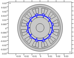
In the Part Libraries window, select AC/DC Module>Rotating Machinery 2D>Rotors>Internal>surface_mounted_magnet_internal_rotor_2d in the tree.
3
Click  Add to Geometry.
Geometry 1
Internal Rotor – Surface Mounted Magnets 1 (pi1)
1
In the Model Builder window, under Component 1 (comp1)>Geometry 1 click Internal Rotor – Surface Mounted Magnets 1 (pi1).
2
In the Settings window for Part Instance, locate the Input Parameters section.
3
4
Click to expand the Domain Selections section. In the table, enter the following settings:
5
Click to expand the Boundary Selections section. In the table, enter the following settings:
Part Libraries
1
In the Home toolbar, click  Windows and choose Part Libraries.
2
In the Model Builder window, click Geometry 1.
3
In the Part Libraries window, select AC/DC Module>Rotating Machinery 2D>Stators>External>slotted_external_stator_2d in the tree.
4
Click  Add to Geometry.
Geometry 1
External Stator – Slotted 1 (pi2)
Specify number of slots and select a radial partition for the slot winding type.
1
In the Model Builder window, under Component 1 (comp1)>Geometry 1 click External Stator – Slotted 1 (pi2).
2
In the Settings window for Part Instance, locate the Input Parameters section.
3
4
Locate the Domain Selections section. In the table, enter the following settings:
Create an assembly from the two geometry objects, connected by a pair boundary.
Form Union (fin)
1
In the Model Builder window, under Component 1 (comp1)>Geometry 1 click Form Union (fin).
2
In the Settings window for Form Union/Assembly, locate the Form Union/Assembly section.
3
From the Action list, choose Form an assembly.
4
In the Home toolbar, click  Build All.
5
Click the  Zoom Extents button in the Graphics toolbar.
Create union selections for the motor iron parts.
Definitions
Iron
1
In the Definitions toolbar, click  Union.
2
In the Settings window for Union, type Iron in the Label text field.
3
Locate the Input Entities section. Under Selections to add, click  Add.
4
In the Add dialog box, in the Selections to add list, choose Rotor iron (Internal Rotor – Surface Mounted Magnets 1) and Stator iron (External Stator – Slotted 1).
5
Next, add materials and assign them to their appropriate domain selections.
Add Material
1
In the Home toolbar, click  Add Material to open the Add Material window.
2
Go to the Add Material window.
3
4
Click Add to Component in the window toolbar.
5
In the tree, select AC/DC>Soft Iron (Without Losses).
6
Click Add to Component in the window toolbar.
7
8
Click Add to Component in the window toolbar.
9
In the tree, select AC/DC>Hard Magnetic Materials>Sintered NdFeB Grades (Chinese Standard)>N54 (Sintered NdFeB).
10
Click Add to Component in the window toolbar.
11
In the tree, select Built-in>Iron.
12
Click Add to Component in the window toolbar.
13
In the Home toolbar, click  Add Material to close the Add Material window.
Materials
Soft Iron (Without Losses) (mat2)
1
In the Model Builder window, under Component 1 (comp1)>Materials click Soft Iron (Without Losses) (mat2).
2
In the Settings window for Material, locate the Geometric Entity Selection section.
3
From the Selection list, choose Iron.
Iron (mat5)
1
In the Model Builder window, click Iron (mat5).
2
In the Settings window for Material, locate the Geometric Entity Selection section.
3
From the Selection list, choose Shaft (Internal Rotor – Surface Mounted Magnets 1).
4
Locate the Material Contents section. In the table, enter the following settings:
Copper (mat3)
1
In the Model Builder window, click Copper (mat3).
2
In the Settings window for Material, locate the Geometric Entity Selection section.
3
From the Selection list, choose Stator slots (External Stator – Slotted 1).
N54 (Sintered NdFeB) (mat4)
1
In the Model Builder window, click N54 (Sintered NdFeB) (mat4).
2
In the Settings window for Material, locate the Geometric Entity Selection section.
3
From the Selection list, choose Rotor magnets (Internal Rotor – Surface Mounted Magnets 1).
Component 1 (comp1)
Rotating Domain 1
1
In the Definitions toolbar, click  Moving Mesh and choose Domains>Rotating Domain.
2
In the Settings window for Rotating Domain, locate the Domain Selection section.
3
From the Selection list, choose All (Internal Rotor – Surface Mounted Magnets 1).
4
Locate the Rotation section. From the Rotation type list, choose Specified rotational velocity.
5
In the ω text field, type w_rot*2*pi.
Rotating Machinery, Magnetic (rmm)
1
In the Model Builder window, under Component 1 (comp1) click Rotating Machinery, Magnetic (rmm).
2
In the Settings window for Rotating Machinery, Magnetic, locate the Thickness section.
3
In the d text field, type L.
B-H Iron Regions
1
In the Physics toolbar, click  Domains and choose Ampère’s Law.
2
In the Settings window for Ampère’s Law, type B-H Iron Regions in the Label text field.
3
Locate the Domain Selection section. From the Selection list, choose Iron.
4
Locate the Constitutive Relation B-H section. From the Magnetization model list, choose B-H curve.
Loss Calculation 1
1
In the Physics toolbar, click  Attributes and choose Loss Calculation.
2
In the Settings window for Loss Calculation, locate the Loss Model section.
3
From the Loss model list, choose Steinmetz.
Conducting Magnet 1
1
In the Physics toolbar, click  Domains and choose Conducting Magnet.
2
In the Settings window for Conducting Magnet, locate the Domain Selection section.
3
From the Selection list, choose Rotor magnets (Internal Rotor – Surface Mounted Magnets 1).
4
Locate the Magnet section. From the Pattern type list, choose Circular pattern.
Loss Calculation 1
In the Physics toolbar, click  Attributes and choose Loss Calculation.
North 1
1
In the Model Builder window, click North 1.
2
South 1
1
In the Model Builder window, click South 1.
2
The Multiphase Winding feature simplifies excitation of stator coils of electrical machines. For three-phase systems an automatic ordering of coil domains into a balanced stator winding is supported, provided that the electrical machine topology in terms of number of poles and slots can accommodate it. In the following steps, use a Multiphase Winding feature to automatically populate the selections of three subnodes with coil domains representing each phase.
Multiphase Winding 1
1
In the Physics toolbar, click  Domains and choose Multiphase Winding.
2
In the Settings window for Multiphase Winding, locate the Domain Selection section.
3
From the Selection list, choose Stator slots (External Stator – Slotted 1).
4
Locate the Multiphase Winding section. In the Ipk text field, type I0.
5
In the αi text field, type init_ang.
6
In the ft text field, type f_el.
7
Locate the Homogenized Multiturn Conductor section. In the N text field, type Nturn.
8
From the Coil wire cross-section area list, choose Filling factor.
9
In the f text field, type ff_slot.
10
Locate the Multiphase Winding section. From the Winding layout configuration list, choose Automatic three phase.
11
In the Number of poles text field, type Np.
12
In the Number of slots text field, type Ns.
13
In the Number of coils per slot text field, type 2.
14
Click Add Phases.
Automatic Phase 1
Selection of the generated phases can be inspected.
Reversed Current Direction 1
Multiphase Winding 1
In the Model Builder window, expand the Automatic Phase 1 node, then click Component 1 (comp1)>Rotating Machinery, Magnetic (rmm)>Multiphase Winding 1.
Loss Calculation 1
In the Physics toolbar, click  Attributes and choose Loss Calculation.
Next, implement the Arkkio Torque Calculation feature for calculating the torque on the rotor. The node is automatically applied to the air gap. The Arkkio force integrand is multiplied with a support function which is nonzero in the correct radial extent, between the rotor magnets and stator iron.
Arkkio Torque Calculation 1
In the Physics toolbar, click  Domains and choose Arkkio Torque Calculation.
Set up a probe for the motor torque.
Definitions
Torque
1
In the Definitions toolbar, click  Probes and choose Global Variable Probe.
2
In the Settings window for Global Variable Probe, type Torque in the Label text field.
3
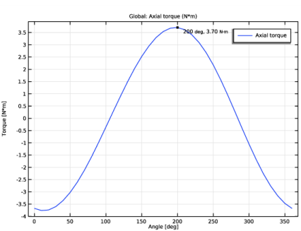
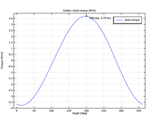
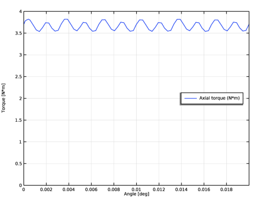
Click Replace Expression in the upper-right corner of the Expression section. From the menu, choose Component 1 (comp1)>Rotating Machinery, Magnetic>Mechanical>rmm.Tark_1 - Axial torque - N·m.
Adjust the default mesh to ensure sufficient resolution of magnetic field in the airgap where torque will be calculated.
Identity Boundary Pair 1 (ap1)
1
In the Model Builder window, click Identity Boundary Pair 1 (ap1).
2
In the Settings window for Pair, locate the Source Boundaries section.
3
Click  Create Selection.
4
In the Create Selection dialog box, type source in the Selection name text field.
5
6
In the Settings window for Pair, locate the Destination Boundaries section.
7
Click  Create Selection.
8
In the Create Selection dialog box, type dest in the Selection name text field.
9
Airgap Boundaries
1
In the Definitions toolbar, click  Union.
2
In the Settings window for Union, type Airgap Boundaries in the Label text field.
3
Locate the Geometric Entity Level section. From the Level list, choose Boundary.
4
Locate the Input Entities section. Under Selections to add, click  Add.
5
In the Add dialog box, in the Selections to add list, choose source and dest.
6
Mesh 1
Size
In the Model Builder window, under Component 1 (comp1) right-click Mesh 1 and choose Edit Physics-Induced Sequence.
Size 1
1
In the Model Builder window, right-click Mesh 1 and choose Size.
2
Drag and drop Size 1 below Size.
3
In the Settings window for Size, locate the Geometric Entity Selection section.
4
From the Geometric entity level list, choose Boundary.
5
From the Selection list, choose Airgap Boundaries.
6
Locate the Element Size section. Click the Custom button.
7
Locate the Element Size Parameters section.
8
Select the Maximum element size check box. In the associated text field, type 0.5[mm]/3.
9
Click  Build All.
10
In the Maximum element size text field, type 0.5[mm]/2.
11
Click  Build All.
Set Linear elements for the discretization. This will yield a more reliable solution near regions of magnetic saturation.
Rotating Machinery, Magnetic (rmm)
1
In the Model Builder window, under Component 1 (comp1) click Rotating Machinery, Magnetic (rmm).
2
In the Settings window for Rotating Machinery, Magnetic, click to expand the Discretization section.
3
From the Magnetic vector potential list, choose Linear.
4
From the Magnetic scalar potential list, choose Linear.
Configure a stationary study to find the electrical angle providing maximum motoring torque.
Study 1: Initial Electrical Angle Sweep
1
In the Model Builder window, click Study 1.
2
In the Settings window for Study, type Study 1: Initial Electrical Angle Sweep in the Label text field.
Step 1: Stationary
1
In the Model Builder window, under Study 1: Initial Electrical Angle Sweep click Step 1: Stationary.
2
In the Settings window for Stationary, click to expand the Study Extensions section.
3
Select the Auxiliary sweep check box.
4
5
Solution 1 (sol1)
1
In the Study toolbar, click  Show Default Solver.
2
In the Model Builder window, expand the Solution 1 (sol1) node.
3
In the Model Builder window, expand the Study 1: Initial Electrical Angle Sweep>Solver Configurations>Solution 1 (sol1)>Stationary Solver 1 node, then click Fully Coupled 1.
4
In the Settings window for Fully Coupled, click to expand the Method and Termination section.
5
In the Maximum number of iterations text field, type 30.
6
In the Model Builder window, collapse the Study 1: Initial Electrical Angle Sweep node.
Monitor the torque while solving by clicking the Probe Plot 1 next to the Graphics window after pushing the Compute-button.
7
In the Study toolbar, click  Compute.
Results
Streamline 1
1
In the Model Builder window, expand the Magnetic Flux Density Norm (rmm) node.
2
Right-click Streamline 1 and choose Disable.
Contour 1
1
In the Model Builder window, click Contour 1.
2
In the Settings window for Contour, locate the Levels section.
3
In the Total levels text field, type 16.
4
Locate the Coloring and Style section. From the Color list, choose Black.
5
In the Magnetic Flux Density Norm (rmm) toolbar, click  Plot.
1D Plot Group 3
In the Home toolbar, click  Add Plot Group and choose 1D Plot Group.
Torque
1
In the Model Builder window, under Results click Probe Plot Group 2.
2
In the Settings window for 1D Plot Group, type Torque in the Label text field.
3
Locate the Plot Settings section.
4
Select the x-axis label check box. In the associated text field, type Angle [deg].
5
Select the y-axis label check box. In the associated text field, type Torque [N*m].
Torque Initial Electrical Angle Sweep
1
In the Model Builder window, under Results click 1D Plot Group 3.
2
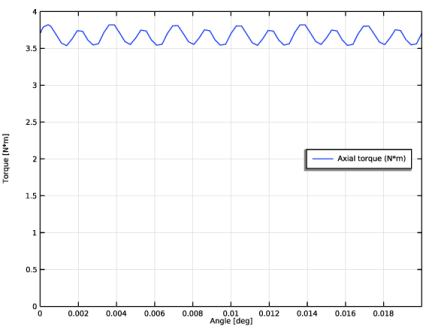
In the Settings window for 1D Plot Group, type Torque Initial Electrical Angle Sweep in the Label text field.
3
Locate the Plot Settings section.
4
Select the x-axis label check box. In the associated text field, type Angle [deg].
5
Select the y-axis label check box. In the associated text field, type Torque [N*m].
Global 1
1
Right-click Torque Initial Electrical Angle Sweep and choose Global.
2
In the Settings window for Global, locate the y-Axis Data section.
3
Graph Marker 1
1
Right-click Global 1 and choose Graph Marker.
2
In the Settings window for Graph Marker, locate the Text Format section.
3
Select the Show x-coordinate check box.
4
Select the Include unit check box.
5
In the Display precision text field, type 3.
6
Locate the Display section. From the Display list, choose Max.
7
In the Torque Initial Electrical Angle Sweep toolbar, click  Plot.
The maximum torque is found at an initial electrical angle offset of 200°. Update init_ang with this value to orient the stator field with respect to rotor magnets so as to achieve maximum torque production.
Global Definitions
Parameters 1
1
In the Model Builder window, under Global Definitions click Parameters 1.
2
In the Settings window for Parameters, locate the Parameters section.
3
In order for the transient solver to achieve a stable solution of the nonlinear problem, set Update Jacobian to On every iteration. This will make the convergence more robust within each time step.
Add Study
1
In the Home toolbar, click  Add Study to open the Add Study window.
2
Go to the Add Study window.
3
Find the Studies subsection. In the Select Study tree, select General Studies>Stationary.
4
Click Add Study in the window toolbar.
5
In the Home toolbar, click  Add Study to close the Add Study window.
Study 2: Synchronous Rotation, Two Electrical Periods
1
In the Model Builder window, click Study 2.
2
In the Settings window for Study, type Study 2: Synchronous Rotation, Two Electrical Periods in the Label text field.
Time Dependent
1
In the Study toolbar, click  Study Steps and choose Time Dependent>Time Dependent.
2
In the Settings window for Time Dependent, locate the Study Settings section.
3
In the Output times text field, type range(0,1/12/6,2)/f_el.
Solution 2 (sol2)
1
In the Study toolbar, click  Show Default Solver.
2
In the Model Builder window, expand the Solution 2 (sol2) node.
3
In the Model Builder window, expand the Study 2: Synchronous Rotation, Two Electrical Periods>Solver Configurations>Solution 2 (sol2)>Stationary Solver 1 node, then click Fully Coupled 1.
4
In the Settings window for Fully Coupled, locate the Method and Termination section.
5
In the Maximum number of iterations text field, type 30.
6
In the Model Builder window, expand the Study 2: Synchronous Rotation, Two Electrical Periods>Solver Configurations>Solution 2 (sol2)>Time-Dependent Solver 1 node, then click Fully Coupled 1.
7
In the Settings window for Fully Coupled, click to expand the Method and Termination section.
8
From the Jacobian update list, choose On every iteration.
9
In the Model Builder window, collapse the Study 2: Synchronous Rotation, Two Electrical Periods node.
10
In the Study toolbar, click  Compute.
Results
Torque Ripple
1
In the Model Builder window, under Results click Torque.
2
In the Settings window for 1D Plot Group, type Torque Ripple in the Label text field.
3
Locate the Axis section. Select the Manual axis limits check box.
4
In the x minimum text field, type 0.
5
In the x maximum text field, type 0.02.
6
In the y minimum text field, type 0.
7
In the y maximum text field, type 4.
8
Locate the Legend section. From the Position list, choose Middle right.
9
In the Torque Ripple toolbar, click  Plot.
Now plot the radial component of the magnetic flux density in the air gap. To do that, define a suitable boundary within the air gap, and plot the quantity along its arc length.
Air Gap Radial Magnetic Flux Density
1
In the Home toolbar, click  Add Plot Group and choose 1D Plot Group.
2
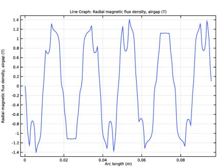
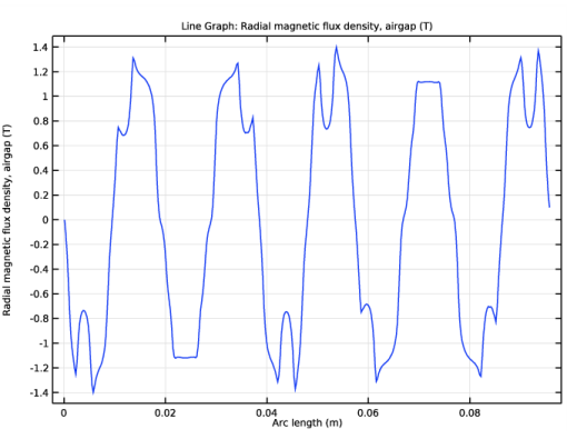
In the Settings window for 1D Plot Group, type Air Gap Radial Magnetic Flux Density in the Label text field.
3
Locate the Data section. From the Dataset list, choose Study 2: Synchronous Rotation, Two Electrical Periods/Solution 2 (sol2).
4
From the Time selection list, choose First.
Line Graph 1
1
Right-click Air Gap Radial Magnetic Flux Density and choose Line Graph.
2
In the Settings window for Line Graph, locate the Selection section.
3
From the Selection list, choose Exterior (Internal Rotor – Surface Mounted Magnets 1).
4
Locate the y-Axis Data section. In the Expression text field, type rmm.ark1.Brad.
5
In the Air Gap Radial Magnetic Flux Density toolbar, click  Plot.
Add Study
1
In the Home toolbar, click  Add Study to open the Add Study window.
2
Go to the Add Study window.
3
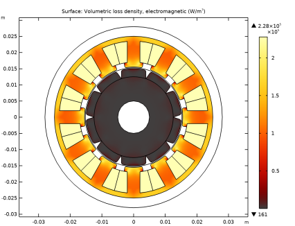
Find the Studies subsection. In the Select Study tree, select Preset Studies for Selected Physics Interfaces>Time to Frequency Losses.
4
Click Add Study in the window toolbar.
5
In the Home toolbar, click  Add Study to close the Add Study window.
Study 3: Loss Calculation over One Electrical Period
1
In the Model Builder window, click Study 3.
2
In the Settings window for Study, type Study 3: Loss Calculation over One Electrical Period in the Label text field.
Step 1: Time to Frequency Losses
1
In the Model Builder window, under Study 3: Loss Calculation over One Electrical Period click Step 1: Time to Frequency Losses.
2
In the Settings window for Time to Frequency Losses, locate the Study Settings section.
3
From the Input study list, choose Study 2: Synchronous Rotation, Two Electrical Periods, Time Dependent.
4
In the Electrical period text field, type 1/f_el.
5
In the Home toolbar, click  Compute.
Results
Cycle Averaged Losses (rmm)
In the Cycle Averaged Losses (rmm) toolbar, click  Plot.
Component 1 (comp1)
In the Model Builder window, collapse the Component 1 (comp1) node.
Results
Torque over One Electrical Period
1
In the Results toolbar, click  Evaluation Group.
2
In the Settings window for Evaluation Group, locate the Data section.
3
From the Dataset list, choose Study 2: Synchronous Rotation, Two Electrical Periods/Solution 2 (sol2).
4
In the Label text field, type Torque over One Electrical Period.
Global Evaluation 1
1
Right-click Torque over One Electrical Period and choose Global Evaluation.
2
In the Settings window for Global Evaluation, locate the Expressions section.
3
Torque over One Electrical Period
1
In the Model Builder window, click Torque over One Electrical Period.
2
In the Settings window for Evaluation Group, locate the Data section.
3
From the Time selection list, choose Interpolated.
4
In the Times (s) text field, type range(1,1/12/6,2)/f_el.
5
In the Torque over One Electrical Period toolbar, click  Evaluate.
Torque Harmonics
1
In the Home toolbar, click  Add Plot Group and choose 1D Plot Group.
2
In the Settings window for 1D Plot Group, type Torque Harmonics in the Label text field.
3
Click to expand the Title section. From the Title type list, choose Manual.
4
In the Title text area, type Torque Harmonics.
Table Graph 1
1
Right-click Torque Harmonics and choose Table Graph.
2
In the Settings window for Table Graph, locate the Data section.
3
From the Source list, choose Evaluation group.
4
From the Transformation list, choose Discrete Fourier transform.
5
From the Show list, choose Frequency spectrum.
6
From the Scale list, choose Multiply by sampling period.
7
Click to expand the Preprocessing section. Find the x-axis column subsection. From the Preprocessing list, choose Linear.
8
In the Scaling text field, type f_el.
9
Locate the Coloring and Style section. From the Width list, choose 2.
10
In the Torque Harmonics toolbar, click  Plot.