|
|
|
|
1
|
|
2
|
In the Select Physics tree, select AC/DC>Magnetic Fields, No Currents>Magnetic Fields, No Currents (mfnc).
|
|
3
|
Click Add.
|
|
4
|
Click
|
|
5
|
|
6
|
Click
|
|
1
|
|
2
|
|
3
|
Click
|
|
4
|
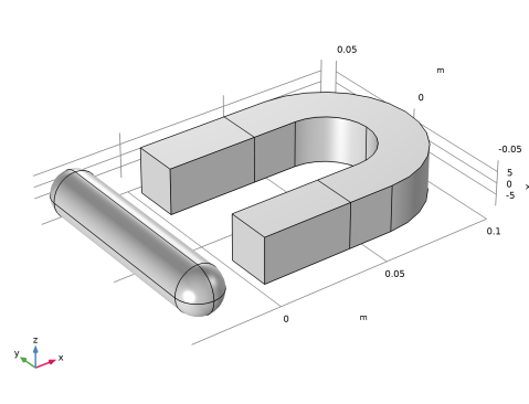
Browse to the model’s Application Libraries folder and double-click the file permanent_magnet.mphbin.
|
|
5
|
|
1
|
|
2
|
|
3
|
|
4
|
|
5
|
|
6
|
|
7
|
|
1
|
|
2
|
Click in the Graphics window and then press Ctrl+A to select both objects.
|
|
3
|
|
4
|
|
5
|
|
6
|
|
1
|
In the Model Builder window, under Component 1 (comp1) right-click Materials and choose Blank Material.
|
|
2
|
|
4
|
|
1
|
|
2
|
|
4
|
|
1
|
|
2
|
|
3
|
In the tree, select AC/DC>Hard Magnetic Materials>Sintered NdFeB Grades (Chinese Standard)>N54 (Sintered NdFeB).
|
|
4
|
|
5
|
|
1
|
|
2
|
|
3
|
|
4
|
Click OK.
|
|
1
|
In the Model Builder window, under Component 1 (comp1) right-click Magnetic Fields, No Currents (mfnc) and choose Magnet.
|
|
1
|
|
1
|
|
1
|
|
2
|
|
4
|
|
5
|
|
1
|
|
3
|
|
4
|
|
1
|
|
2
|
|
3
|
|
1
|
|
2
|
|
3
|
|
5
|
|
6
|
|
7
|
|
8
|
|
1
|
|
2
|
|
3
|
|
4
|
|
1
|
|
2
|
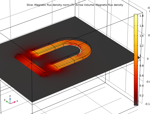
In the Settings window for Slice, click Replace Expression in the upper-right corner of the Expression section. From the menu, choose Component 1 (comp1)>Magnetic Fields, No Currents>Magnetic>mfnc.normB - Magnetic flux density norm - T.
|
|
3
|
|
4
|
|
5
|
|
6
|
|
7
|
|
8
|
Click OK.
|
|
9
|
|
1
|
|
2
|
In the Settings window for Arrow Volume, click Replace Expression in the upper-right corner of the Expression section. From the menu, choose Component 1 (comp1)>Magnetic Fields, No Currents>Magnetic>mfnc.Bx,...,mfnc.Bz - Magnetic flux density.
|
|
3
|
Locate the Arrow Positioning section. Find the x grid points subsection. In the Points text field, type 100.
|
|
4
|
|
5
|
|
6
|
|
7
|
|
1
|
|
2
|
|
3
|
|
1
|
|
2
|
|
3
|
|
4
|
|
5
|
|
1
|
|
2
|
|
3
|
|
4
|
|
1
|
|
2
|
In the Settings window for Arrow Volume, click Replace Expression in the upper-right corner of the Expression section. From the menu, choose Component 1 (comp1)>Magnetic Fields, No Currents>Magnetic>mfnc.Bx,...,mfnc.Bz - Magnetic flux density.
|
|
3
|
|
1
|
|
2
|
In the Settings window for Global Evaluation, click Replace Expression in the upper-right corner of the Expressions section. From the menu, choose Component 1 (comp1)>Magnetic Fields, No Currents>Mechanical>Electromagnetic force - N>mfnc.Forcex_rod - Electromagnetic force, x-component.
|
|
3
|
|
4
|
|
5
|
Click
|