PDF

Magnetic Prospecting of Iron Ore Deposits
Introduction
Magnetic prospecting is one of the methods of geological exploration applicable to certain types of iron ore deposits, in particular those made up of magnetite and hematite. Estimates of center-of-mass coordinates and the spatial extent of iron-rich layers help decrease the cost of exploration. Passive magnetic prospecting relies on accurate mapping of local geomagnetic anomalies — deviations of the natural magnetostatic fields from their predicted values based on the magnetic dipole model of Earth’s field. This application investigates magnetic anomaly estimation for both surface and aerial prospecting.
Crustal magnetic anomalies may result from either induced or remnant magnetization of iron-rich rocks. Among all terrestrial iron minerals, magnetite has the largest magnetic permeability (up to μr = 650 in small-grain magnetite) and the strongest naturally occurring thermo-remnant magnetization (up to Mr = 5000 A/m) (Ref. 1). Another mineral with relatively strong magnetization is hematite (Ref. 1). Magnetite and hematite are the major minerals of high-grade iron ore. This application uses modest values of magnetic permeability (μr = 3.5) and remnant magnetization (Mr = 60 A/m) that are typical for terrestrial magnetite with a grain size distribution of 20200 μm (Ref. 1). The concentration of magnetite in the iron-rich ore is assumed to be 25%.
Model Definition
Magnetostatic problems without significant electrical currents can be solved in terms of a scalar magnetic potential. Variations of the magnetic permeability or remnant magnetization cause small deviations of magnetic fields from the norm (local geomagnetic anomalies), which you can model accurately using the reduced potential formulation of the Magnetic Fields, No Currents interface. The background magnetic field is assumed to be uniform within the simulation domain. Intensity and orientation of the natural magnetic field is estimated using the data from National Geophysical Data Center of the U.S. Government (Ref. 2).
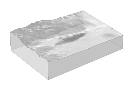
This application neglects the induced and remnant magnetization of the rocks outside the iron ore body. The iron ore bed is approximated by a uniform flat ellipsoid with a maximum vertical thickness of 100 m, a maximum North-South width of 400 m, and an East-West extent of 2000 m. Center-of-mass coordinates of the ore bed (25001500) meters from the lower-left corner (200 meters above sea level) are positioned underneath the Eastern Pit of the Eagle Mountain Mine, a former Kaiser Steel Co. mining operation in Riverside County, California (Ref. 3). The specific location and shape of magnetic ore in this application are not based on any actual geological prospecting but are chosen to simulate a basic size and shape of such an ore. Figure 1 shows the model geometry.
Figure 1: The model geometry.
Topography
The topographical map used for this application consists of a rectangular grid containing 157-by-111 points spaced 1 arc second (1/3600°) apart in both horizontal directions. The curvature of the geoid is neglected in drawing this geometry from elevation data. The lower-left (south-west) corner of the map is located at a latitude 33.85° (North) and longitude 115.5° (West). The size of the simulation domain is 4836 m in an East-West (x-axis), 3410 m in a North-South direction (y-axis), and 1934.4 m in the up-down direction (z-axis). A satellite image of this area can be seen in (Ref. 4).
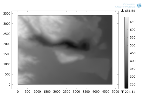
A digital elevation model (DEM) for this example can be derived from the National Elevation Dataset (NED) of the U.S. Geological Survey data center (Ref. 5). The free program MicroDEM (Ref. 6) converts the USGS elevation data into an ASCII file containing the elevation matrix, which you can import into COMSOL Multiphysics as an Interpolation function feature. From the interpolation function you can then create a geometry by using a Parametric Surface feature. Optionally, the resulting geometry can be saved in the internal binary CAD file format (.mphbin). Importing the saved CAD file into the COMSOL Desktop is the starting point for the step-by-step instructions for this application. Figure 2 contains a plot of the resulting elevation map as it appears in COMSOL Multiphysics.
Figure 2: Elevation map of the simulation domain (boundary plot of z-coordinate on Boundary 6).
Domain Equations
In a current-free region, where
it is possible to define a scalar magnetic potential, Vm, such that
This is analogous to the definition of the electric potential for static electric fields. Using the constitutive relation between the magnetic flux density and magnetic field,
together with the equation
one can derive an equation for Vm:
The reduced potential formulation used in this model splits the total magnetic potential into external and reduced parts, Vtot = Vext + Vred, where the reduced potential Vred is the dependent variable:
The external magnetic potential is more easily defined as an external magnetic field, so the equation that is used in practice is rather
To simulate the background geomagnetic field, components of the external magnetic field are expressed through total intensity, magnetic declination, and inclination angles as follows:
Based on the data provided by NOAA’s data center (Ref. 3), inclination and declination angles for this location (N 33.85°, W 115.5°) are approximately Incl = 59.357° and Decl = 12.275°, respectively. The magnitude of natural magnetic flux density (Bμ0H0) is estimated as 48.163 μT.
Remnant magnetic flux density is assumed to be aligned with the local contemporary direction of geomagnetic field:
In general, thermo-remnant magnetization does not have to be aligned with Earth’s magnetic field.
The values of magnetic permeability and remnant flux used for the iron ore are based on the typical parameters of magnetite ore and a simple homogenization model taking into account dilution of magnetization in the ore bed:
Concentration of magnetite cmagn in the ore is assumed to be 25%.
Boundary Conditions
Along the exterior boundaries of the surrounding box, the perturbation of the magnetic field (Hred) is assumed to be tangential to the boundaries. The natural boundary condition from the equation is
Thus, the reduced magnetic field is made tangential to the boundary by a Neumann condition on the reduced potential. Interior boundaries are modeled as continuity boundary conditions and require no user input.
The Magnetic Fields, No Currents interface automatically adds a point constraint, Vm = 0, using a weak term on the equation-system level if there are no boundary conditions that constrain the value of Vm (such as Magnetic potential or Zero potential). This ensures that the scalar potential Vm is uniquely defined in problems with pure Neumann boundary conditions.
Results and Discussion
Figure 3 shows deviations of the magnetic field intensity on the ground (boundary plot), and at an altitude of 1300 meters. The maximum magnetic field perturbation on the ground is 2 A/m and at 1300 meters altitude it has fallen to 0.1 A/m. In both locations the maximum is located approximately above the center of mass of the magnetite ore body. These results show that aerial magnetic prospecting may reveal the location and provide estimates of the horizontal extent of magnetite-rich deposits but also that ground-based magnetic prospecting apparently is a much more sensitive exploration tool than aerial prospecting.
Figure 3: The slice color plot shows perturbations of magnetic intensity (norm of reduced magnetic field) at an altitude 1300 m. The boundary plot shows the same quantity on the ground.
Figure 4: Arrows show the direction and relative magnitude of the reduced magnetic field on Earth’s surface.
Figure 5 shows a slice plot of the dimensionless ratio of remanent and induced magnetizations, Br/(μ0M), inside the iron ore body, at an elevation of 200 m above sea level. This plot indicates that contributions of remanent and induced magnetizations to the magnetic anomaly can be comparable for realistic magnetic parameters of magnetite (Ref. 1).
Figure 5: Slice plot of the dimensionless ratio of remanent to induced magnetizations inside the iron ore body at an elevation of 200 m above sea level. The two contributions to the magnetic anomaly are of comparable magnitude.
References
1. G. Kletetschka, P.J. Wasilewski, and P.T. Taylor, “Hematite vs. magnetite as the signature for planetary magnetic anomalies”, Physics of the Earth and Planetary Interiors, vol. 119, pp. 259–267, 2000.
2. NOAA, National Centers for Environmental Information, https://www.ngdc.noaa.gov/geomag-web/
3. E.R. Force, “Eagle Mountain Mine – Geology of the former Kaiser Steel operation in Riverside county, California”, U.S. Geological Survey Open-File Report 01-237.
4. Google Maps, https://maps.google.com/maps?f=q&hl=en&geocode=&q=33.865,-115.475&ie=UTF8&t=h&z=16&iwloc=addr
5. Data available from U.S. Geological Survey, National Elevation Data set, using The National Map Advanced Viewer, https://viewer.nationalmap.gov/advanced-viewer/
6. MICRODEM Home Page, http://www.usna.edu/Users/oceano/pguth/website/microdem/microdem.htm
Application Library path: ACDC_Module/Introductory_Magnetostatics/magnetic_prospecting
Modeling Instructions
From the File menu, choose New.
New
In the New window, click  Model Wizard.
Model Wizard
1
In the Model Wizard window, click  3D.
2
In the Select Physics tree, select AC/DC>Magnetic Fields, No Currents>Magnetic Fields, No Currents (mfnc).
3
Click Add.
4
Click  Study.
5
In the Select Study tree, select General Studies>Stationary.
6
Global Definitions
Parameters 1
1
In the Model Builder window, under Global Definitions click Parameters 1.
2
In the Settings window for Parameters, locate the Parameters section.
3
Variables 1
1
In the Home toolbar, click  Variables and choose Global Variables.
2
In the Settings window for Variables, locate the Variables section.
3
Geometry 1
The geometry obtained from the heightmap is available in an MPHBIN-file (COMSOL Multiphysics’ native CAD file format) that can be imported in the geometry node.
Import 1 (imp1)
1
In the Home toolbar, click  Import.
2
In the Settings window for Import, locate the Import section.
3
Click  Browse.
4
5
Click  Import.
Create an ellipsoid that models the iron ore deposit.
Ellipsoid 1 (elp1)
1
In the Geometry toolbar, click  More Primitives and choose Ellipsoid.
2
In the Settings window for Ellipsoid, locate the Size and Shape section.
3
In the a-semiaxis text field, type 1000.
4
In the b-semiaxis text field, type 200.
5
In the c-semiaxis text field, type 50.
6
Locate the Position section. In the x text field, type 2500.
7
In the y text field, type 1500.
8
In the z text field, type 200.
9
Click  Build All Objects.
Activate the transparency to verify that the deposit is in the correct position.
10
Click the  Transparency button in the Graphics toolbar.
Materials
Use one material for the background (air and nonmagnetic rocks) and another for the iron ore. For the ore, you specify the relative permeability as a material property but add the remanent magnetization in the physics settings.
Background Material
1
In the Model Builder window, under Component 1 (comp1) right-click Materials and choose Blank Material.
2
In the Settings window for Material, locate the Material Contents section.
3
4
In the Label text field, type Background Material.
Ore
1
Right-click Materials and choose Blank Material.
2
3
In the Settings window for Material, locate the Material Contents section.
4
5
In the Label text field, type Ore.
Magnetic Fields, No Currents (mfnc)
Magnetic Flux Conservation 2
1
In the Model Builder window, under Component 1 (comp1) right-click Magnetic Fields, No Currents (mfnc) and choose Magnetic Flux Conservation.
2
3
In the Settings window for Magnetic Flux Conservation, locate the Constitutive Relation B-H section.
4
From the Magnetization model list, choose Remanent flux density.
5
From the  ||  Br   ||  list, choose User defined. In the associated text field, type Br.
6
Specify the e vector as
Specify the local geomagnetic field as the background field for the problem.
7
In the Model Builder window, click Magnetic Fields, No Currents (mfnc).
8
In the Settings window for Magnetic Fields, No Currents, locate the Background Magnetic Field section.
9
From the Solve for list, choose Reduced field.
10
Specify the Hb vector as
External Magnetic Flux Density 1
1
In the Physics toolbar, click  Boundaries and choose External Magnetic Flux Density.
Apply External Magnetic Flux Density as the boundary condition instead of Magnetic Insulation. The former operates only on the relative field, while the latter sets a condition for the total field.
2
Study 1
Disable the automatic generation of the default plots. You will manually create the plots after the solution.
1
In the Model Builder window, click Study 1.
2
In the Settings window for Study, locate the Study Settings section.
3
Clear the Generate default plots check box.
4
In the Home toolbar, click  Compute.
Results
In the Model Builder window, expand the Results node.
Create a second solution with a selection active only on the boundary corresponding to the Earth’s surface. You will use this solution when plotting surface data.
Study 1/Solution 1 (2) (sol1)
1
In the Model Builder window, expand the Results>Datasets node.
2
Right-click Results>Datasets and choose Solution.
Selection
1
In the Results toolbar, click  Attributes and choose Selection.
2
In the Settings window for Selection, locate the Geometric Entity Selection section.
3
From the Geometric entity level list, choose Boundary.
4
3D Plot Group 1
In the Results toolbar, click  3D Plot Group.
Surface 1
1
Right-click 3D Plot Group 1 and choose Surface.
2
In the Settings window for Surface, locate the Data section.
3
From the Dataset list, choose Study 1/Solution 1 (2) (sol1).
4
Click Replace Expression in the upper-right corner of the Expression section. From the menu, choose Component 1 (comp1)>Magnetic Fields, No Currents>Magnetic>mfnc.normredH - Reduced magnetic field norm - A/m.
5
Locate the Expression section. In the Expression text field, type down(mfnc.normredH).
6
Select the Description check box. In the associated text field, type Reduced magnetic field norm (downside).
The down() operator indicates in this case that the value on the ground side should be used, not the default mean of the values on each side.
7
In the 3D Plot Group 1 toolbar, click  Plot.
3D Plot Group 1
The plot of the relative magnetic field at the altitude of 1300 m can be obtained with a simple slice plot.
Slice 1
1
In the Model Builder window, right-click 3D Plot Group 1 and choose Slice.
2
In the Settings window for Slice, locate the Plane Data section.
3
From the Plane list, choose xy-planes.
4
From the Entry method list, choose Coordinates.
5
In the z-coordinates text field, type 1300.
6
Click Replace Expression in the upper-right corner of the Expression section. From the menu, choose Component 1 (comp1)>Magnetic Fields, No Currents>Magnetic>mfnc.normredH - Reduced magnetic field norm - A/m.
7
Locate the Coloring and Style section. Click  Change Color Table.
8
In the Color Table dialog box, select Thermal>GrayBody in the tree.
9
10
In the 3D Plot Group 1 toolbar, click  Plot.
The plot shows the alteration of the geomagnetic field due to the presence of a magnetized material. Note how the relative magnetic field intensity at ground level is about 20 times larger than at 1300 m.
11
Click the  Transparency button in the Graphics toolbar to return to the default state.
Next, add another plot group to visualize the vector field.
3D Plot Group 2
In the Home toolbar, click  Add Plot Group and choose 3D Plot Group.
Add a uniform gray surface representing the ground.
Surface 1
Right-click 3D Plot Group 2 and choose Surface.
3D Plot Group 2
1
In the Settings window for 3D Plot Group, locate the Data section.
2
From the Dataset list, choose Study 1/Solution 1 (2) (sol1).
Surface 1
1
In the Model Builder window, click Surface 1.
2
In the Settings window for Surface, locate the Expression section.
3
In the Expression text field, type 0.
4
Locate the Coloring and Style section. From the Coloring list, choose Uniform.
5
From the Color list, choose Gray.
3D Plot Group 2
Now plot the relative magnetic field at ground level.
Arrow Surface 1
1
In the Model Builder window, right-click 3D Plot Group 2 and choose Arrow Surface.
2
In the Settings window for Arrow Surface, click Replace Expression in the upper-right corner of the Expression section. From the menu, choose Component 1 (comp1)>Magnetic Fields, No Currents>Magnetic>mfnc.redHx,...,mfnc.redHz - Reduced magnetic field.
3
Locate the Arrow Positioning section. In the Number of arrows text field, type 2000.
4
In the 3D Plot Group 2 toolbar, click  Plot.
5
Click the  Zoom In button in the Graphics toolbar.
The plot shows the vector field for the magnetic field perturbation caused by the iron ore deposit.
Finally, plot the ratio between the remanent flux density and the induced magnetization.
3D Plot Group 3
In the Home toolbar, click  Add Plot Group and choose 3D Plot Group.
Slice 1
1
Right-click 3D Plot Group 3 and choose Slice.
2
In the Settings window for Slice, locate the Plane Data section.
3
From the Plane list, choose xy-planes.
4
From the Entry method list, choose Coordinates.
5
In the z-coordinates text field, type 200.
6
Locate the Expression section. In the Expression text field, type mfnc.normBr/(mu0_const*mfnc.normM).
7
In the 3D Plot Group 3 toolbar, click  Plot.
The plot shows that the two contributions are comparable in magnitude.
8
Click the  Go to Default View button in the Graphics toolbar.