PDF

Hartmann Boundary Layer
Introduction
The velocity profile of a Hartmann boundary layer is a classical Magnetohydrodynamics problem with an analytical solution, making it appropriate for benchmarking of numerical models. This model consists of an electrically conducting liquid flowing between two no-slip surfaces immersed in an externally applied constant magnetic field. The electromotive force, as seen in the fluid frame of reference, induces a volumetric current, which in turn generates a Lorentz force opposing the flow velocity.
Model Definition
The model is set up in 2D using the Magnetic Fields and Laminar Flow physics interfaces, coupled via a Magnetohydrodynamics multiphysics node.
Analytical Solution
The flow profile between the two plates can be found if the material properties are assumed constant, and the no-slip condition is applied at both walls. The velocity is
where U = u/U0 is the velocity u normalized to the average inlet velocity U0, Y = y/d is the position normalized to the distance between the no-slip planes 2d, and the Hartmann number Ha = μH0d is the ratio of electromagnetic to viscous forces where μ is the magnetic permeability, H0 the imposed magnetic field strength, σ the electrical conductivity, ρ the mass density, and the kinematic viscosity.
Results
Figure 1 compares the simulation results for three different values of the Hartmann number with the corresponding analytic solutions.
Figure 2 shows the absolute error of the numeric solution for the normalized velocity for the same Hartmann number values.
Figure 1: The normalized velocity profiles for three magnitudes of the Hartmann number plotted as functions of the y-coordinate compared with the corresponding analytical values.
Figure 2: The absolute error of the normalized velocity plotted as a function of the y-coordinate for three magnitudes of the Hartmann number.
Application Library path: ACDC_Module/Electromagnetics_and_Fluids/hartmann_boundary_layer
Modeling Instructions
From the File menu, choose New.
New
In the New window, click  Model Wizard.
Model Wizard
1
In the Model Wizard window, click  2D.
2
In the Select Physics tree, select AC/DC>Electromagnetics and Fluids>Magnetohydrodynamics, Out-of-Plane Currents.
3
Click Add.
4
Click  Study.
5
In the Select Study tree, select General Studies>Stationary.
6
Global Definitions
Parameters 1
1
In the Model Builder window, under Global Definitions click Parameters 1.
2
In the Settings window for Parameters, locate the Parameters section.
3
Velocity profile
1
In the Home toolbar, click  Functions and choose Global>Analytic.
2
In the Settings window for Analytic, type Velocity profile in the Label text field.
3
In the Function name text field, type an_U.
4
Locate the Definition section. In the Expression text field, type (cosh(Ha)-cosh(Ha*Y))/(cosh(Ha)-1/Ha*sinh(Ha)).
5
In the Arguments text field, type Ha, Y.
6
Locate the Plot Parameters section. In the table, enter the following settings:
Geometry 1
Rectangle 1 (r1)
1
In the Geometry toolbar, click  Rectangle.
2
In the Settings window for Rectangle, locate the Size and Shape section.
3
In the Width text field, type 80*d.
4
In the Height text field, type 2*d.
5
Locate the Position section. In the y text field, type -d.
6
In the Geometry toolbar, click  Build All.
Materials
Fluid
1
In the Model Builder window, under Component 1 (comp1) right-click Materials and choose Blank Material.
2
In the Settings window for Material, type Fluid in the Label text field.
3
Locate the Material Contents section. In the table, enter the following settings:
Laminar Flow (spf)
Inlet 1
1
In the Model Builder window, under Component 1 (comp1) right-click Laminar Flow (spf) and choose Inlet.
2
3
In the Settings window for Inlet, locate the Boundary Condition section.
4
From the list, choose Fully developed flow.
5
Clear the Apply condition on each disjoint selection separately check box.
6
Locate the Fully Developed Flow section. In the Uav text field, type U0.
Outlet 1
1
In the Physics toolbar, click  Boundaries and choose Outlet.
2
Magnetic Fields (mf)
1
In the Model Builder window, under Component 1 (comp1) click Magnetic Fields (mf).
2
In the Settings window for Magnetic Fields, locate the Background Field section.
3
From the Solve for list, choose Reduced field.
4
From the Background field specification list, choose Uniform magnetic flux density.
5
Specify the Bb vector as
External Magnetic Vector Potential 1
1
In the Physics toolbar, click  Boundaries and choose External Magnetic Vector Potential.
2
Click in the Graphics window and then press Ctrl+A to select all boundaries.
Mesh 1
Mapped 1
In the Mesh toolbar, click  Mapped.
Distribution 1
Right-click Mapped 1 and choose Distribution.
Size 1
In the Model Builder window, right-click Mapped 1 and choose Size.
Distribution 1
1
2
In the Settings window for Distribution, locate the Distribution section.
3
From the Distribution type list, choose Predefined.
4
In the Number of elements text field, type 50.
5
In the Element ratio text field, type 20.
6
Select the Symmetric distribution check box.
Size 1
1
In the Model Builder window, click Size 1.
2
In the Settings window for Size, locate the Element Size section.
3
Click the Custom button.
4
Locate the Element Size Parameters section.
5
Select the Maximum element size check box. In the associated text field, type d.
6
Click  Build Selected.
Study 1
Step 1: Stationary
1
In the Model Builder window, under Study 1 click Step 1: Stationary.
2
In the Settings window for Stationary, click to expand the Study Extensions section.
3
Select the Auxiliary sweep check box.
4
5
6
In the Home toolbar, click  Compute.
Results
Streamline 1
1
In the Model Builder window, expand the Magnetic Flux Density Norm (mf) node, then click Streamline 1.
2
In the Settings window for Streamline, locate the Streamline Positioning section.
3
In the Separating distance text field, type 0.015.
4
In the Magnetic Flux Density Norm (mf) toolbar, click  Plot.
Velocity (spf)
1
In the Model Builder window, under Results click Velocity (spf).
2
In the Settings window for 2D Plot Group, locate the Data section.
3
From the Parameter value (Ha) list, choose 1.
4
In the Velocity (spf) toolbar, click  Plot.
5
Click the  Zoom Extents button in the Graphics toolbar.
Contour
1
In the Model Builder window, expand the Pressure (spf) node.
2
Right-click Contour and choose Disable.
Surface 1
1
In the Model Builder window, right-click Pressure (spf) and choose Surface.
2
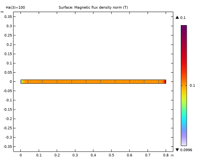
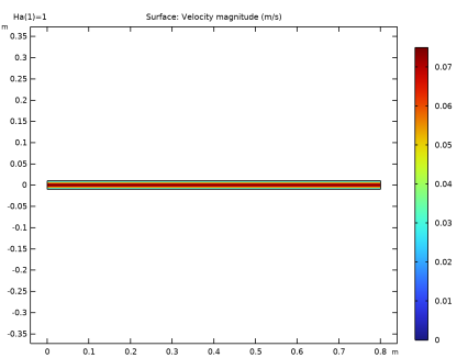
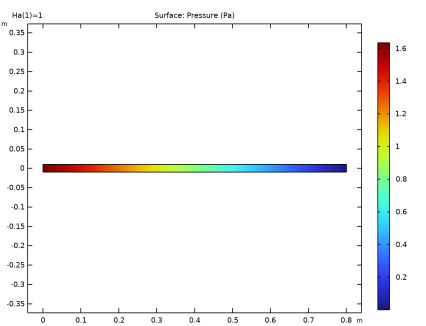
In the Settings window for Surface, click Replace Expression in the upper-right corner of the Expression section. From the menu, choose Component 1 (comp1)>Laminar Flow>Velocity and pressure>p - Pressure - Pa.
3
In the Pressure (spf) toolbar, click  Plot.
Pressure (spf)
1
In the Model Builder window, click Pressure (spf).
2
In the Settings window for 2D Plot Group, locate the Data section.
3
From the Parameter value (Ha) list, choose 1.
4
In the Pressure (spf) toolbar, click  Plot.
5
Click the  Zoom Extents button in the Graphics toolbar.
Longitudinal section
1
In the Model Builder window, expand the Results>Datasets node.
2
Right-click Results>Datasets and choose Cut Line 2D.
3
In the Settings window for Cut Line 2D, type Longitudinal section in the Label text field.
4
Locate the Line Data section. In row Point 2, set x to 80*d.
Cross section
1
In the Results toolbar, click  Cut Line 2D.
2
In the Settings window for Cut Line 2D, locate the Line Data section.
3
In row Point 1, set x to 70*d.
4
In row Point 1, set y to -d.
5
In row Point 2, set x to 70*d.
6
In row Point 2, set y to d.
7
In the Label text field, type Cross section.
Normalized velocity on the center line
1
In the Results toolbar, click  1D Plot Group.
2
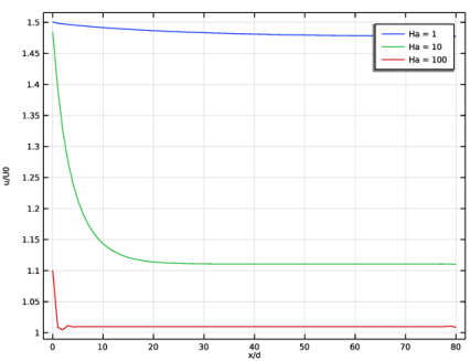
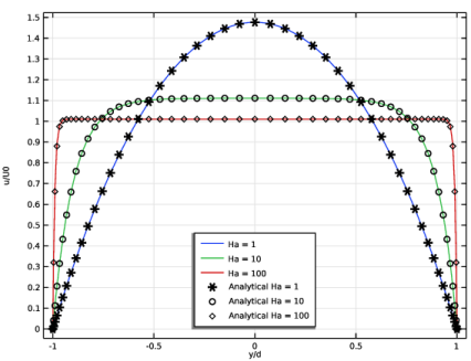
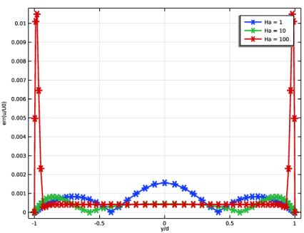
In the Settings window for 1D Plot Group, type Normalized velocity on the center line in the Label text field.
3
Locate the Data section. From the Dataset list, choose Longitudinal section.
4
Locate the Plot Settings section.
5
Select the x-axis label check box. In the associated text field, type x/d.
6
Select the y-axis label check box. In the associated text field, type u/U0.
Line Graph 1
1
Right-click Normalized velocity on the center line and choose Line Graph.
2
In the Settings window for Line Graph, locate the Data section.
3
From the Dataset list, choose Longitudinal section.
4
Locate the y-Axis Data section. In the Expression text field, type u/U0.
5
Locate the x-Axis Data section. From the Parameter list, choose Expression.
6
In the Expression text field, type x/d.
7
Click to expand the Legends section. Select the Show legends check box.
8
Find the Prefix and suffix subsection. In the Prefix text field, type Ha = .
9
Click to expand the Title section. From the Title type list, choose None.
10
Click the  Zoom Extents button in the Graphics toolbar.
Normalized velocity profiles
1
In the Results toolbar, click  1D Plot Group.
2
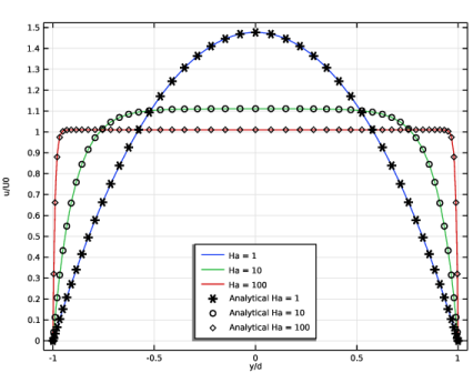
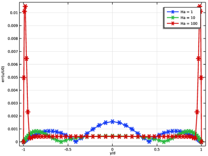
In the Settings window for 1D Plot Group, type Normalized velocity profiles in the Label text field.
3
Locate the Data section. From the Dataset list, choose Cross section.
4
Locate the Plot Settings section. Select the x-axis label check box.
5
Select the y-axis label check box.
6
In the x-axis label text field, type y/d.
7
In the y-axis label text field, type u/U0.
8
Locate the Legend section. From the Position list, choose Lower middle.
Line Graph 1
1
Right-click Normalized velocity profiles and choose Line Graph.
2
In the Settings window for Line Graph, locate the y-Axis Data section.
3
In the Expression text field, type u/U0.
4
Locate the x-Axis Data section. From the Parameter list, choose Expression.
5
In the Expression text field, type y/d.
6
Locate the Legends section. Select the Show legends check box.
7
Find the Prefix and suffix subsection. In the Prefix text field, type Ha = .
8
Locate the Title section. From the Title type list, choose None.
Line Graph 2
1
In the Model Builder window, right-click Normalized velocity profiles and choose Line Graph.
2
In the Settings window for Line Graph, locate the y-Axis Data section.
3
In the Expression text field, type an_U(Ha,y/d).
4
Locate the x-Axis Data section. From the Parameter list, choose Expression.
5
In the Expression text field, type y/d.
6
Locate the Legends section. Select the Show legends check box.
7
Find the Prefix and suffix subsection. In the Prefix text field, type Analytical Ha = .
8
Click to expand the Coloring and Style section. Find the Line style subsection. From the Line list, choose None.
9
From the Color list, choose Black.
10
Find the Line markers subsection. From the Marker list, choose Cycle.
11
Click to expand the Quality section. From the Resolution list, choose No refinement.
12
From the Smoothing list, choose None.
13
Locate the Title section. From the Title type list, choose None.
14
In the Normalized velocity profiles toolbar, click  Plot.
15
Click the  Zoom Extents button in the Graphics toolbar.
Normalized velocity error
1
In the Home toolbar, click  Add Plot Group and choose 1D Plot Group.
2
In the Settings window for 1D Plot Group, type Normalized velocity error in the Label text field.
3
Locate the Data section. From the Dataset list, choose Cross section.
4
Locate the Plot Settings section.
5
Select the x-axis label check box. In the associated text field, type y/d.
6
Select the y-axis label check box. In the associated text field, type err(u/U0).
Line Graph 1
1
Right-click Normalized velocity error and choose Line Graph.
2
In the Settings window for Line Graph, locate the y-Axis Data section.
3
In the Expression text field, type abs(u/U0-an_U(Ha, y/d)).
4
Locate the x-Axis Data section. From the Parameter list, choose Expression.
5
In the Expression text field, type y/d.
6
Locate the Coloring and Style section. From the Width list, choose 2.
7
Find the Line markers subsection. From the Marker list, choose Asterisk.
8
Locate the Legends section. Select the Show legends check box.
9
Find the Prefix and suffix subsection. In the Prefix text field, type Ha = .
10
Locate the Quality section. From the Resolution list, choose No refinement.
11
From the Smoothing list, choose None.
12
Locate the Title section. From the Title type list, choose None.
13
In the Normalized velocity error toolbar, click  Plot.
14
Click the  Zoom Extents button in the Graphics toolbar.