PDF

Hall Effect Sensor
Introduction
The Hall effect sensor is commonly used for position and proximity sensing. A current is applied across a conducting piece of metal, and in the presence of a magnetic field perpendicular to the current direction, the charge carriers experience a Lorentz force. Owing to current conservation, this force is counterbalanced by charge accumulation building up an electric field. In the stationary case, a voltage drop proportional to the magnetic field applied to the conductor can therefore be measured.
Model Definition
The model is set up in 3D by one-way coupling the Electric Currents interface to the Magnetic Fields, No Currents interface where the constitutive relation for the conduction current in the former takes into account the magnetic flux density as given by the latter. It is also assumed that the current in the sensor is small enough that the resulting current-induced magnetic field can be neglected. With this current-free assumption, the magnetic field can be described via the gradient of a scalar magnetic potential, and a two-way coupled non-linear problem is avoided.
Hall Effect via Anisotropic Conductivity
The conduction current constitutive relation is:
where Jc, E, and B, in turn, represent the conduction current, the electric field, and the magnetic field. Furthermore, σ and Rh denote the isotropic electrical conductivity and the Hall coefficient, respectively. Representing the cross product with a matrix multiplication
the current density can be related to the electric field via an anisotropic conductivity tensor , which is defined by
where I is the identity matrix. The Hall effect option for the conduction model implements this anisotropic conductivity tensor and requires the isotropic conductivity, the Hall coefficient, and the magnetic flux density as model inputs.
Results
Figure 1 displays the electric potential in the sensor conductor and the magnetic flux density generated by the permanent magnet, with the magnitude and direction of the magnetic field indicated by arrows.
Figure 2 shows the electric potential drop perpendicular to the sensor current direction, as a function of the magnet position.
Figure 1: Electric potential plotted in the sensor, and magnetic flux density generated by the permanent magnet. The arrows indicate the magnitude and direction of the magnetic field.
Figure 2: Electric potential drop between the two floating surfaces, plotted as a function of the wheel angle.
Application Library path: ACDC_Module/Devices,_Capacitive/hall_effect_sensor
Modeling Instructions
From the File menu, choose New.
New
In the New window, click  Model Wizard.
Model Wizard
1
In the Model Wizard window, click  3D.
2
In the Select Physics tree, select AC/DC>Electric Fields and Currents>Electric Currents (ec).
3
Click Add.
4
In the Select Physics tree, select AC/DC>Magnetic Fields, No Currents>Magnetic Fields, No Currents (mfnc).
5
Click Add.
6
Click  Study.
7
In the Select Study tree, select General Studies>Stationary.
8
Global Definitions
Parameters 1
1
In the Model Builder window, under Global Definitions click Parameters 1.
2
In the Settings window for Parameters, locate the Parameters section.
3
Geometry 1
Work Plane 1 (wp1)
1
In the Model Builder window, expand the Component 1 (comp1)>Geometry 1 node.
2
Right-click Geometry 1 and choose Work Plane.
3
In the Settings window for Work Plane, locate the Plane Definition section.
4
In the z-coordinate text field, type -12.5[mm].
Work Plane 1 (wp1)>Plane Geometry
In the Model Builder window, click Plane Geometry.
Work Plane 1 (wp1)>Rectangle 1 (r1)
1
In the Work Plane toolbar, click  Rectangle.
2
In the Settings window for Rectangle, locate the Size and Shape section.
3
In the Width text field, type 1[cm].
4
In the Height text field, type 5[mm].
5
Locate the Position section. From the Base list, choose Center.
Work Plane 1 (wp1)>Rectangle 2 (r2)
1
In the Work Plane toolbar, click  Rectangle.
2
In the Settings window for Rectangle, locate the Size and Shape section.
3
In the Width text field, type 1[mm].
4
In the Height text field, type 7[mm].
5
Locate the Position section. From the Base list, choose Center.
Work Plane 1 (wp1)>Union 1 (uni1)
1
In the Work Plane toolbar, click  Booleans and Partitions and choose Union.
2
Click in the Graphics window and then press Ctrl+A to select both objects.
3
In the Settings window for Union, locate the Union section.
4
Clear the Keep interior boundaries check box.
Work Plane 1 (wp1)>Fillet 1 (fil1)
1
In the Work Plane toolbar, click  Fillet.
2
On the object uni1, select Points 4, 5, 8, and 9 only.
3
In the Settings window for Fillet, locate the Radius section.
4
In the Radius text field, type 1[mm].
Work Plane 1 (wp1)>Plane Geometry
In the Work Plane toolbar, click  Build All.
Extrude 1 (ext1)
1
In the Model Builder window, right-click Geometry 1 and choose Extrude.
2
In the Settings window for Extrude, locate the Distances section.
3
Cylinder 1 (cyl1)
1
In the Geometry toolbar, click  Cylinder.
2
In the Settings window for Cylinder, locate the Size and Shape section.
3
In the Radius text field, type 2[mm].
4
In the Height text field, type 1[mm].
5
Locate the Position section. In the z text field, type -10.5[mm].
Cylinder 2 (cyl2)
1
In the Geometry toolbar, click  Cylinder.
2
In the Settings window for Cylinder, locate the Size and Shape section.
3
In the Radius text field, type 10[mm].
4
In the Height text field, type 6[mm].
5
Locate the Position section. In the y text field, type -3[mm].
6
Locate the Axis section. From the Axis type list, choose y-axis.
Union 1 (uni1)
1
In the Geometry toolbar, click  Booleans and Partitions and choose Union.
2
Click the  Zoom Extents button in the Graphics toolbar.
3
Click the  Wireframe Rendering button in the Graphics toolbar.
4
Select the objects cyl1 and cyl2 only.
5
In the Settings window for Union, click  Build Selected.
Delete Entities 1 (del1)
1
Right-click Geometry 1 and choose Delete Entities.
2
On the object uni1, select Boundary 10 only.
Sphere 1 (sph1)
1
In the Geometry toolbar, click  Sphere.
2
In the Settings window for Sphere, locate the Size section.
3
In the Radius text field, type 25[mm].
4
Click to expand the Layers section. In the table, enter the following settings:
5
In the Geometry toolbar, click  Build All.
Definitions
Set up an infinite element domain surrounding the sensor setup, to remove the influence of the magnetic insulation boundary condition.
Infinite Element Domain 1 (ie1)
1
In the Definitions toolbar, click  Infinite Element Domain.
2
3
In the Settings window for Infinite Element Domain, locate the Geometry section.
4
From the Type list, choose Spherical.
Definitions
The rotation of the magnet is done in two steps: first a General Extrusion maps the vector field to its rotated coordinates, and then a local vector rotation is performed by defining new magnetic field variables.
General Extrusion 1 (genext1)
1
In the Definitions toolbar, click  Nonlocal Couplings and choose General Extrusion.
2
In the Settings window for General Extrusion, locate the Source Selection section.
3
From the Selection list, choose All domains.
4
In the Operator name text field, type rotY.
5
Locate the Destination Map section. In the x-expression text field, type x*cos(Angle)-z*sin(Angle).
6
In the z-expression text field, type x*sin(Angle)+z*cos(Angle).
Variables 1
1
In the Model Builder window, right-click Definitions and choose Variables.
2
In the Settings window for Variables, locate the Variables section.
3
Add Material
1
In the Home toolbar, click  Add Material to open the Add Material window.
2
Go to the Add Material window.
3
4
Click Add to Component in the window toolbar.
5
In the tree, select Built-in>Iron.
6
Click Add to Component in the window toolbar.
7
In the tree, select AC/DC>Hard Magnetic Materials>Sintered NdFeB Grades (Chinese Standard)>N54 (Sintered NdFeB).
8
Click Add to Component in the window toolbar.
9
In the Home toolbar, click  Add Material to close the Add Material window.
Materials
Conductor
1
In the Model Builder window, under Component 1 (comp1) right-click Materials and choose Blank Material.
2
In the Settings window for Material, type Conductor in the Label text field.
3
4
Locate the Material Contents section. In the table, enter the following settings:
Iron (mat2)
1
In the Model Builder window, click Iron (mat2).
2
N54 (Sintered NdFeB) (mat3)
1
In the Model Builder window, click N54 (Sintered NdFeB) (mat3).
2
Electric Currents (ec)
1
In the Model Builder window, under Component 1 (comp1) click Electric Currents (ec).
2
In the Settings window for Electric Currents, locate the Domain Selection section.
3
Click  Clear Selection.
4
Ground 1
1
In the Physics toolbar, click  Boundaries and choose Ground.
2
Terminal 1
1
In the Physics toolbar, click  Boundaries and choose Terminal.
2
3
In the Settings window for Terminal, locate the Terminal section.
4
From the Terminal type list, choose Voltage.
5
In the V0 text field, type 5.
Floating Potential 1
1
In the Physics toolbar, click  Boundaries and choose Floating Potential.
2
Floating Potential 2
1
In the Physics toolbar, click  Boundaries and choose Floating Potential.
2
Magnetic Fields, No Currents (mfnc)
In the Model Builder window, under Component 1 (comp1) click Magnetic Fields, No Currents (mfnc).
Magnet 1
1
In the Physics toolbar, click  Domains and choose Magnet.
2
North 1
1
In the Model Builder window, click North 1.
2
South 1
1
In the Model Builder window, click South 1.
2
Mesh 1
Free Tetrahedral 1
1
In the Mesh toolbar, click  Free Tetrahedral.
2
In the Settings window for Free Tetrahedral, locate the Domain Selection section.
3
From the Geometric entity level list, choose Domain.
4
Swept 1
1
In the Mesh toolbar, click  Swept.
2
In the Settings window for Swept, click to expand the Source Faces section.
3
4
Click to expand the Destination Faces section. Select Boundaries 5–8, 35, 36, 46, and 51 only.
Distribution 1
Right-click Swept 1 and choose Distribution.
Size
1
In the Settings window for Size, locate the Element Size section.
2
From the Predefined list, choose Finer.
3
In the Model Builder window, right-click Mesh 1 and choose Build All.
Magnetic Fields, No Currents (mfnc)
Zero Magnetic Scalar Potential 1
1
In the Physics toolbar, click  Points and choose Zero Magnetic Scalar Potential.
2
Study 1
Solution 1 (sol1)
1
In the Study toolbar, click  Show Default Solver.
2
In the Model Builder window, expand the Solution 1 (sol1) node.
3
In the Model Builder window, expand the Study 1>Solver Configurations>Solution 1 (sol1)>Stationary Solver 1 node.
4
Right-click Study 1>Solver Configurations>Solution 1 (sol1)>Stationary Solver 1>Direct and choose Enable.
5
In the Study toolbar, click  Compute.
Results
Electric Potential (ec)
Global Evaluation 1
1
In the Results toolbar, click  Global Evaluation.
2
In the Settings window for Global Evaluation, locate the Expressions section.
3
4
Clicknext to  Evaluate, then choose New Table.
Electric Currents (ec)
Current Conservation 1
1
In the Model Builder window, under Component 1 (comp1)>Electric Currents (ec) click Current Conservation 1.
2
In the Settings window for Current Conservation, locate the Constitutive Relation Jc-E section.
3
From the Conduction model list, choose Hall effect.
4
In the RH text field, type Rh.
5
Specify the B vector as
Study 1
Step 1: Stationary
1
In the Model Builder window, under Study 1 click Step 1: Stationary.
2
In the Settings window for Stationary, click to expand the Study Extensions section.
3
Select the Auxiliary sweep check box.
4
5
Results
Magnet
1
In the Model Builder window, expand the Results>Electric Potential (ec) node.
2
Right-click Electric Potential (ec) and choose Volume.
3
In the Settings window for Volume, type Magnet in the Label text field.
4
Locate the Expression section. In the Expression text field, type 1.
5
Locate the Coloring and Style section. From the Coloring list, choose Uniform.
6
From the Color list, choose Gray.
Transparency 1
1
Right-click Magnet and choose Transparency.
2
In the Settings window for Transparency, locate the Transparency section.
3
In the Transparency text field, type 0.1.
Selection 1
1
In the Model Builder window, right-click Magnet and choose Selection.
2
Deformation 1
1
Right-click Magnet and choose Deformation.
2
In the Settings window for Deformation, locate the Expression section.
3
In the x-component text field, type -rotY(x)-x.
4
In the y-component text field, type 0.
5
In the z-component text field, type rotY(z)-z.
6
Locate the Scale section.
7
Select the Scale factor check box. In the associated text field, type 1.
Electric Potential and Magnetic Flux Density Norm
1
In the Model Builder window, under Results click Electric Potential (ec).
2
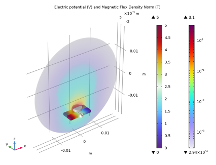
In the Settings window for 3D Plot Group, type Electric Potential and Magnetic Flux Density Norm in the Label text field.
3
Click to expand the Title section. From the Title type list, choose Manual.
4
In the Title text area, type Electric potential (V) and Magnetic Flux Density Norm (T).
5
Locate the Plot Settings section. Clear the Plot dataset edges check box.
Slice 1
Right-click Electric Potential and Magnetic Flux Density Norm and choose Slice.
Selection 1
1
In the Model Builder window, right-click Slice 1 and choose Selection.
2
Slice 1
1
In the Model Builder window, click Slice 1.
2
In the Settings window for Slice, locate the Plane Data section.
3
From the Plane list, choose zx-planes.
4
In the Planes text field, type 1.
5
Locate the Expression section. In the Expression text field, type sqrt(rBx^2 + rBy^2 + rBz^2).
6
Select the Description check box. In the associated text field, type Magnetic Flux Density Norm.
7
In the Electric Potential and Magnetic Flux Density Norm toolbar, click  Plot.
8
Click to expand the Range section. Select the Manual color range check box.
9
Locate the Coloring and Style section. From the Scale list, choose Logarithmic.
10
Click  Change Color Table.
11
In the Color Table dialog box, select Rainbow>Prism in the tree.
12
Transparency 1
Right-click Slice 1 and choose Transparency.
Electric Potential and Magnetic Flux Density Norm
Add a contour line for the electric potential to visualize the influence of the magnet.
Contour 1
1
In the Model Builder window, right-click Electric Potential and Magnetic Flux Density Norm and choose Contour.
2
In the Settings window for Contour, locate the Levels section.
3
From the Entry method list, choose Levels.
4
In the Levels text field, type 2.5.
5
Locate the Coloring and Style section. From the Coloring list, choose Uniform.
6
From the Color list, choose Black.
7
Clear the Color legend check box.
8
Click to expand the Title section. From the Title type list, choose None.
Selection 1
1
Right-click Contour 1 and choose Selection.
2
Electric Potential and Magnetic Flux Density Norm
1
In the Model Builder window, under Results click Electric Potential and Magnetic Flux Density Norm.
2
In the Electric Potential and Magnetic Flux Density Norm toolbar, click  Plot.
3
Click the  Zoom Extents button in the Graphics toolbar.
Study 1
Step 1: Stationary
1
In the Model Builder window, under Study 1 click Step 1: Stationary.
2
In the Settings window for Stationary, click to expand the Results While Solving section.
3
Select the Plot check box.
4
In the Home toolbar, click  Compute.
Results
Global Evaluation 1
In the Model Builder window, under Results>Derived Values right-click Global Evaluation 1 and choose Evaluate>New Table.
Sensor Potential Difference
1
In the Home toolbar, click  Add Plot Group and choose 1D Plot Group.
2
In the Settings window for 1D Plot Group, type Sensor Potential Difference in the Label text field.
3
Locate the Plot Settings section.
4
Select the y-axis label check box. In the associated text field, type Sensor Potential Drop.
Table Graph 1
1
Right-click Sensor Potential Difference and choose Table Graph.
2
In the Settings window for Table Graph, locate the Data section.
3
From the Table list, choose Table 2.
4
In the Sensor Potential Difference toolbar, click  Plot.