Single-Phase Flow
The Fluid Flow>Single-Phase Flow branch () when adding a physics interface includes the Laminar and Creeping Flow interfaces.
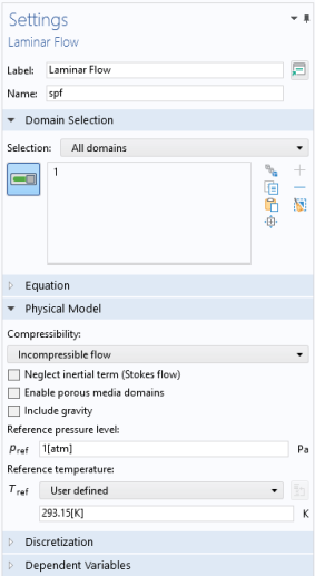
The Laminar Flow Interface () is used primarily to model slow-moving flow in environments without sudden changes in geometry, material distribution, or temperature. The Navier-Stokes equations are solved without a turbulence model. Laminar flow typically occurs at Reynolds numbers less than 1000. By default the flow is incompressible (see Figure 2-1).
The Creeping Flow Interface () uses the same equations as the Laminar Flow interface with the additional assumption that the contribution of the inertia term is negligible. This is often referred to as Stokes flow and is appropriate for use when viscous flow is dominant, which is often the case in microfluidics applications. Creeping flow applies when the Reynolds number is much less than one. A creeping flow problem is significantly simpler to solve than a laminar flow problem — so it is best to make this assumption explicitly if it applies. By default the flow is incompressible (see below).
By selecting the Neglect Inertial Form (Stokes Flow) check box, on the Settings window for Laminar Flow quickly convert a Laminar Flow interface into a Creeping Flow interface.
For both physics interfaces several additional options are available.
Shallow Channel Approximation
Often you might want to simplify long, narrow channels by modeling them in 2D. The Use Shallow Channel Approximation option is useful as it includes a drag term to approximate the added affects given by thinness of the gap between one set of boundaries in comparison to the others.
Compressible Flow
For compressible flow it is important that the density and any mass balances are well defined throughout the domain. Choosing to model incompressible flow simplifies the equations to be solved and decreases solution times. Most gas flows should be modeled as compressible flows; however, liquid flows can usually be treated as incompressible.
Include gravity
Gravity can be included when required. It can be neglected in models dominated by other effects.
Non-Newtonian Flow
The physics interfaces also allow for easy definition of non-Newtonian fluid flow through access to the dynamic viscosity in the Navier–Stokes equations. The fluid can be modeled using the Power law, Carreau, Bingham–Papanastasiou, Herschel–Bulkley–Papanastasiou, and Casson–Papanastasiou models or by means of any expression that describes the dynamic viscosity appropriately. To use other non-Newtonian models or model viscoelastic flow, the Polymer Flow Module is recommended in addition to the Microfluidics Module. The different non-Newtonian models can be defined directly in the physics, or using the corresponding Material Model nodes.
Both physics interfaces also include a feature to compute a laminar velocity profile at arbitrarily shaped inlets and outlets, which makes models much easier to set up.
Figure 2-1: The Settings window for Laminar Flow. Model incompressible or compressible (Ma<0.3) flow, and Stokes flow. Combinations are also possible.