You are viewing the documentation for an older COMSOL version. The latest version is available here.
Parameterized TTT Diagram
A curve in a TTT diagram represents the time it takes to form a certain relative phase fraction of a metallurgical phase, under isothermal conditions. Using experimental TTT diagram data, one can extract transformations times across a range of temperatures and thereby characterize temperature dependent phase transformations. This is what you typically need to do for the TTT Diagram Data formulations of the Leblond-Devaux, the JMAK, and the Kirkaldy-Venugopalan phase transformation models. In some situations, it may be sufficient to approximate the shape of a TTT curve using analytical functions. COMSOL Multiphysics provides a functionality to enter three characteristic time-temperature points on a TTT curve, and together with two shape parameters, construct an approximate a TTT curve. The three points that are used to define the TTT curve in this way are:
The points are designated U (upper), L (lower), and N (nose), see Figure 3-4.
Figure 3-4: A parameterized TTT curve.
The parameterized TTT curve is defined by two analytical functions that meet at the nose. They are:
,
,
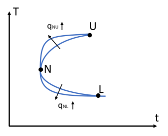
The shape parameters qNL and qNU are used to control the shape of the curve below the nose (NL) and above the nose (NU), and the effect of increasing them is schematically shown in Figure 3-4. A shape parameter value of two produces a quadratic function in the log time - temperature space, and so on. When you parameterize the curves in a TTT diagram in this way, COMSOL Multiphysics will internally use the TTT curves in the same way as if you had used the TTT Diagram Data formulations.