In general, as the length scale (L) of the device is reduced, the scaling of a physical effect with respect to L determines its relative importance. The inertial force required to produce a fixed acceleration of a solid body scales volumetrically as L3. The scaling of other forces in comparison to this inertial force has important consequences for MEMS devices. For example, the effective spring constant for a body scales as L1. The spring stiffness therefore decreases much more slowly than the system mass as the size of the system is reduced, resulting in higher resonant frequencies for smaller devices (resonant frequency scales as L−1). This means that micromechanical systems typically have higher operating frequencies and faster response times than macroscopic systems.

Electrostatic forces scale favorably as the device dimensions are reduced (for example, the force between parallel plates with a fixed applied voltage scales as L0). Additionally, electrostatic actuators consume no DC power and can be manufactured using processes that are compatible with standard semiconductor foundries. Many MEMS devices utilize electrostatic actuation for this reason.

Piezoelectric forces also scale well as the device dimension is reduced (the force produced by a constant applied voltage scales as L1). Furthermore, piezoelectric sensors and actuators are predominantly linear and do not consume DC power in operation. Piezoelectrics are more difficult to integrate with standard semiconductor processes, but significant progress has been made with commercial successes in the market (for example, FBAR filters). Quartz frequency references can be considered the highest volume MEMS component currently in production with more than 1 billion (1·109) devices manufactured per year. Although not traditionally considered to be within the MEMS umbrella (the quartz industry long predates the coining of the term), many of these devices have mm to sub-mm dimensions and are lithographically defined. Furthermore, some quartz products are now being branded as MEMS devices.

The following figure shows the mechanical response of a thickness shear quartz oscillator, together with a graph showing the effect of a series capacitance (Cs) on the frequency response. A series capacitance is frequently used to tune or pull the resonance of quartz oscillators.

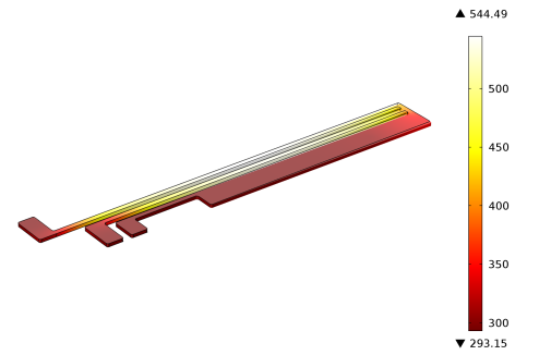
Thermal forces scale as L2, assuming that the forces are generated by a fixed temperature change. This scaling is still favorable in comparison to inertial forces, and the thermal time scale also scales well (as L2), making thermal actuators faster on the microscale (although thermal actuators are typically slower than capacitive or piezoelectric actuators). Thermal actuators are also easy to integrate with semiconductor processes although they usually consume large amounts of power and thus have had a limited commercial applicability. Thermal effects play an important role in the manufacture of many commercial MEMS technologies with thermal stresses in deposited thin films being critical for many applications. The following figure shows the temperature within a displaced, Joule-heated actuator.

Fluidic MEMS devices, or microfluidic devices, represent an increasingly important area of MEMS. COMSOL provides a separate Microfluidics Module to specifically address these applications. Nonetheless, the MEMS Module includes significant microfluidic functionality for simulating the interaction of MEMS structures with fluids. One area of significant interest is that of thin-film damping. Damping forces scale as L1 and are often important for MEMS devices, frequently leading to a requirement for vacuum packaging. The figure below shows the pressure on the surface of a simple accelerometer. This pressure results from the compression of the thin layer of rarefied gas between the accelerometer and the package (the package is not shown in the figure).

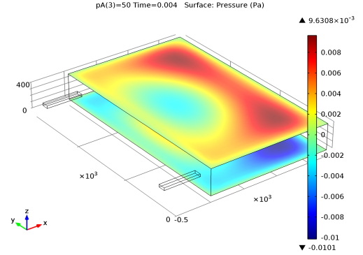
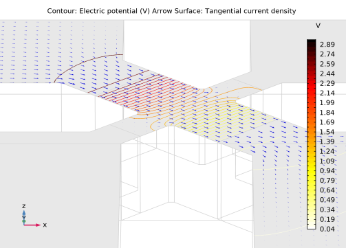
The preceding discussion has focused on the forces available for driving actuators, but scaling is also important for the operation of sensors. Piezoresistive sensors typically produce an output proportional to stress, which for a fixed strain scales independently of device dimension (as L0). The piezoresistive effect refers to the change in a material’s conductivity that occurs in response to an applied stress. The ease of integration of small piezoresistors with standard semiconductor processes, along with the reasonably linear response of the sensor, has made this technology particularly important in the pressure sensor industry. The following figure shows the current distribution and the induced voltage in a piezoresistor that senses the deflection of a pressure sensor.

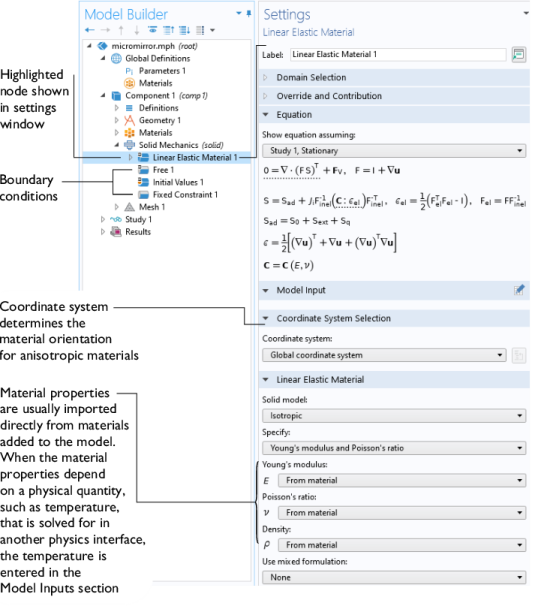
The MEMS physics interfaces are used to simulate MEMS devices. Each physics interface expresses the relevant physical phenomena in the form of sets of partial or ordinary differential equations, together with appropriate boundary and initial conditions. Each feature added to the physics interface represents a term or condition in the underlying equation set. These features are usually associated with a geometric entity within the model, such as a domain, boundary, edge (for 3D components), or point. Figure 1 uses the Micromirror model (found in the MEMS Module application library) to show the Model Builder and the Settings window for the selected Linear Elastic Material 1 feature node. This node adds the equations of structural mechanics to the simulation within the domains selected. Under the Linear Elastic Material section several settings indicate that the Young’s modulus, Poisson’s ratio, and density are inherited from the material properties assigned to the domain. The material properties can be set up as functions of other dependent variables in the model, such as temperature. The Free and Fixed boundary conditions are also indicated in the model tree. The Free boundary condition is applied by default to all surfaces in the model and allows free motion of the surface. The Fixed boundary condition is used to constrain surfaces that are held in place, for example, by attachment to the wafer handle.

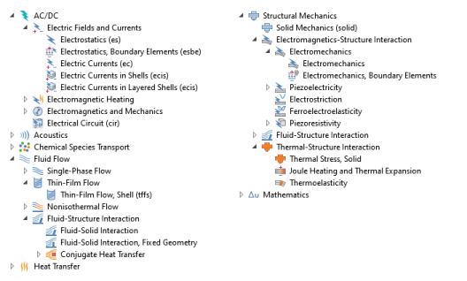
The MEMS Module includes a number of physics interfaces to enable modeling of different physical situations encountered in microsystem design. When a new model is started, these physics interfaces are selected from the Model Wizard. Figure 2 shows the Model Wizard with the physics interfaces included with the MEMS Module. Since MEMS is a multidisciplinary industry, the physics interfaces are spread over a number of different areas within COMSOL’s supported physics types and correspondingly appear on several branches of the Model Wizard. Also see Physics Interface Guide by Space Dimension and Preset Study Type. Below, a brief overview of each of the MEMS Module physics interfaces is given.

The Solid Mechanics interface () defines the quantities and features for stress analysis and general linear and nonlinear solid mechanics, solving for the displacements. The Linear Elastic Material node is the default material model. In addition, the elastic material model can be extended with thermal expansion, viscoelasticity, damping, and initial stress and strain features. The description of elastic materials in the module includes isotropic, orthotropic, and fully anisotropic materials. A number of preset study types are available—see the list in Physics Interface Guide by Space Dimension and Preset Study Type.