The Multibody Dynamics (mbd) interface (), found under the Structural Mechanics branch () when adding a physics interface, is intended for analysis of mechanical assemblies. The parts in the assembly can be rigid or flexible, and are connected by various types of joints, gears, chains, springs, or dampers. Flexible parts can be defined using solid, shell, or beam elements. There are many types of joints, such as hinges or ball joints, which can be used based on the type of connection required between components. There are many types of gears, such as spur, helical, bevel, worm, or rack, which can be used for power transmission. Computed results are displacements, velocities, accelerations, joint forces, gear contact forces, and — in flexible parts — stresses. The joints can be given properties such as spring constants, damping, friction, and limits on movement. The gears pairs can also be given properties such as gear mesh stiffness, mesh damping, backlash, transmission error, and friction.

The Linear Elastic Material is the default material model. It adds the equations for the displacements in a linear elastic solid and has a Settings window to define the elastic and inertia properties of a material. As an alternative, a domain can be made into a rigid body, using the Rigid Material material model. A rigid domain adds the rigid body dynamics equations and has a Settings window to define inertia properties of a material.

When the Multibody Dynamics interface is added, these default nodes are also added to the Model Builder — Linear Elastic Material, Free (a boundary condition where boundaries are free, with no loads or constraints), and Initial Values (only applicable for flexible domains). Then, from the Physics toolbar, add features that implement other multibody dynamics properties. You can also right-click Multibody Dynamics to select physics features from the context menu.

The Label is the default physics interface name.

The Name is used primarily as a scope prefix for variables defined by the physics interface. Refer to such physics interface variables in expressions using the pattern <name>.<variable_name>. In order to distinguish between variables belonging to different physics interfaces, the name string must be unique. Only letters, numbers, and underscores (_) are permitted in the Name field. The first character must be a letter.

The default Name (for the first physics interface in the model) is mbd.

From the Structural transient behavior list, select Include inertial terms or Quasi static. Use Quasi static to treat the mechanical behavior as quasi static (with no mass effects — that is, no second-order time derivatives). Selecting this option gives a more efficient solution for problems where the variation in time is slow when compared to the natural frequencies of the system.

Specify initial values for a rigid body translation and rotation. The values specified here are, as a default, inherited by the initial values settings for Rigid Material and Linear Elastic Material.

By using the Physics Node Generation button (), you can automatically create Rigid Material, Gear, and Joint nodes.

The Physics Node Generation has the following options:

The Create Rigid Domains option () automatically creates Rigid Material nodes for geometrically disconnected objects. The Rigid Domain Selections input controls for which geometric objects to create a rigid domain. It is by default set to From physics interface, which creates rigid domain for all objects in the selection of the physics interface. All available domain selections are also listed in the Rigid Domain Selections list, which makes it possible to create rigid domains for a subset of objects. Select the Include mass and moment of inertia node check box to add a Mass and Moment of Inertia subnode to each auto-generated Rigid Material node. The Density of the created rigid materials is automatically set to zero when this check box is selected.

The Create Gears option () automatically creates a Gear node for every gear geometry part present in the geometry sequence. This option requires that the gear geometry is built from the Multibody Dynamics Module Part Library. The domain selection for the auto-generated Gear node is same as the gear geometry part. Relevant definitions and parameters are retrieved from the gear geometry part, and entered in the settings for the corresponding gear node. The Rigid Domain Selections and Include mass and moment of inertia does not affect the Create Gears option.

The Create Joints option () automatically creates Joint nodes from the geometry based on the shape of the boundaries. This option requires Identity Boundary Pair nodes created under Definitions. If the Source Boundaries and Destination Boundaries are of same standard shape, this option creates one Joint node for each active Identity Boundary Pair present. The possible shapes of boundaries for automatic joint creation are listed under Joint types.

You can select a Body defining reference frame from the list of all rigid domains, attachments, and gears used in the model. It is used to visualize the relative motion of objects with respect to the selected body.

The variables u_ref, v_ref, and w_ref, being the three components of the displacement field with respect to the reference body, are available in the result menus. Also, the variables mbd.disp_ref and mbd.vel_ref contain the total displacement and velocity with respect to the reference body, respectively.

When you change the reference body, you need to update the solution before you can access the new definitions of these variables. To do that, right-click the Study node and select Update Solution () (or press F5).

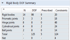
The last two rows of the table contain a summary. In the Total row, the number of DOFs, prescribed conditions, and constraints are summed.

The Net row contains the net number of degrees of freedom of the model — that is, the difference between all degrees of freedom and the constraints and prescribed motions. A negative net number of degrees of freedom indicates that the mechanism is overconstrained and is not shown. In that case, the net number of constraints is instead displayed.

To display this section, click the Show More Options button () and select Advanced Physics Options in the Show More Options dialog box. Normally these settings do not need to be changed.

Select the Rigid connectors check box to group the variables added by Rigid Connector nodes.

Select the Attachments check box to group the variables added by Attachment nodes.

The selection made in this section can be overridden by the settings in the Advanced section of the individual Rigid Connector or Attachment nodes.

In the Multibody Dynamics interface you can choose not only the order of the discretization, but also the type of shape functions: Lagrange or serendipity. For highly distorted elements, Lagrange shape functions provide better accuracy than serendipity shape functions of the same order. The serendipity shape functions, however, give significant reductions of the model size for a given mesh containing hexahedral, prism, or quadrilateral elements.

The discretization order applies to the flexible bodies. The default is to use Linear shape functions for the Displacement field. If you want to compute stresses with good accuracy, increase the shape function order to Quadratic serendipity or Quadratic.

The physics interface uses the global spatial components of the Displacement field u as dependent variables in the flexible domains. The default names for the components are (u, v, w) in 3D. In 2D the component names are (u, v), and in 2D axial symmetry they are (u, w). You can, however, not use the “missing” component name in the 2D cases as a parameter or variable name because it is still used internally.