View Factor Evaluation

The strategy for evaluating view factors is central to any radiation simulation. Loosely speaking, a view factor is a measure of how much influence the radiosity at a given part of the boundary has on the irradiation at some other part.

The quantities Gm and Famb in Equation 4-109 are not strictly view factors in the traditional sense. Instead, Famb is the view factor of the ambient portion of the field of view, which is considered to be a single boundary with constant radiosity

On the other hand, Gm is the integral over all visible points of a differential view factor, multiplied by the radiosity of the corresponding source point. In the discrete model, think of it as the product of a view factor matrix and a radiosity vector. This is, however, not necessarily the way the calculation is performed.

Consider a point P on a surface as in Figure 4-21. It can be seen by points on other surfaces such as S′ in the figure, as well as the ambient surrounding, Samb. Assume that the points on S′ have a local radiosity, J′, while the ambient surrounding has a constant temperature, Tamb.

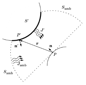
The mutual irradiation at point P is given by the following surface integral:

The heat flux that arrives from P′ depends on the local radiosity J′ projected onto P. The projection is computed using the normal vectors n and n′ along with the vector r, which points from P to P′.

The ambient view factor, Famb, is determined from the integral of the surrounding surfaces S′, here denoted as F′:

The two last equations plug into Equation 4-108 to yield the final equation for irradiative flux.

The equations used so far apply to the general 3D case. 2D geometries result in simpler integrals. For the 2D case, the resulting equations for the mutual irradiation and ambient view factor are

where the integral over S⊥′ denotes the line integral along the boundaries of the 2D geometry.

In axisymmetric geometries or when a symmetry plane is defined, the irradiation and ambient view factor cannot be computed directly from a closed-form expression. Instead, a virtual geometry must be constructed, and the view factors evaluated according to Equation 4-115. For cases with specularly reflective surfaces, specular view factors depends also on specular reflectivities of surrounding surfaces, see Ref. 23.

A separate evaluation is performed for each unique point where Gm or Famb is requested, typically for each quadrature point during solution. Differential view factors are normally computed only once, the first time they are needed, and then stored in memory until next time the model definition or the mesh is changed.

The Heat Transfer Module supports the following surface-to-surface radiation methods, which are selected in the Radiation Settings section in a Heat Transfer interface:

	View factors are always calculated directly from the mesh, which is a polygonal representation of the geometry. To improve the accuracy of the radiative heat transfer simulation, the mesh must be refined rather than raising the element order.

In 3D, the view factor for a point at finite distance is given by

where θ is the angle between the normal to the irradiated surface and the direction of the source, and r is the distance from the source. For a source at infinity, the view factor is given by cos θ.

In 2D the view factor for a point at finite distance is given by

and the view factor for a source at infinity is cos θ.

The Sun is the most common example of an external radiation source. The position of the Sun is necessary to determine the direction of the corresponding external radiation source. The direction of sunlight (zenith angle and the solar elevation) is automatically computed from the latitude, longitude, time zone, date, and time using similar a method as described in Ref. 20. The estimated solar position is accurate for a date between year 2000 and 2199, due to an approximation used in the Julian Day calendar calculation.

The zenith angle, θs, and azimuth angle,

, of the Sun are converted into a direction vector is = (isx, isy, isz) in Cartesian coordinates assuming that the north, the west, and the up directions correspond to the x, y, and z directions, respectively, in the model. The relation between θs,

, and is is given by:

For an axisymmetric geometry, Gm and Famb must be evaluated in a corresponding 3D geometry obtained by revolving the 2D boundaries around the axis. COMSOL Multiphysics creates this virtual 3D geometry by revolving the 2D boundary mesh into a 3D mesh. The resolution can be controlled in the azimuthal direction by setting the number of azimuthal sectors, which is the same as the number of elements to a full revolution. Try to balance this number against the mesh resolution in the rz-plane. This number, the azimuthal sectors, is accessible from the Radiation Settings section in physics interfaces for heat transfer.

Select between the hemicube, the ray shooting and the direct area integration methods also in axial symmetry. Their settings work the same way as in 3D.

	While Gm and Famb are in fact evaluated in a full 3D, the number of points where they are requested is limited to the quadrature points on the boundary of a 2D geometry. The savings compared to a full 3D simulation are therefore substantial despite the full 3D view factor code being used.

The fluence rate is evaluated at a point P, as in Figure 4-21, using the following surface integral:

where S′ corresponds to all the surfaces which can be seen from point P. J′ is the radiosity emitted by the surface S′ in P direction. r is the vector which points from P to P′ located on S′.