Apparent Heat Capacity Method

The apparent heat capacity formulation provides an implicit capturing of the phase change interface, by solving for both phases a single heat transfer equation with effective material properties. The latent heat of phase change is taken into account by modifying the heat capacity.

It applies well to materials showing a mushy zone around the phase change interface. And it allows topology changes of the phase change interface.

The Phase Change Material domain condition should be used on both phases domains, to solve the heat equation after specifying the properties of the phase change material according to the apparent heat capacity formulation.

Instead of adding a latent heat L in the energy balance equation exactly when the material reaches its phase change temperature Tpc, it is assumed that the transformation occurs in a temperature interval ΔT. Within this interval, the material is transformed from phase 1 to phase 2. The corresponding volume fractions of the phases are represented by the phase transition function α 1 → 2, where θ1 = 1 − α 1 → 2 is the volume fraction of the material before transition and θ2 = α 1 → 2 the volume fraction of the material after transition. See the section Phase Transition Function for details about the form of α 1 → 2.

The density, ρ, and the specific enthalpy, H, are expressed by:

Differentiating with respect to temperature, this equality provides the following formula for the specific heat capacity:

which becomes, after some formal transformations:

The mass fraction, αm, is defined from ρ1, ρ2 and θ1, θ2 according to:

The specific heat capacity is the sum of an equivalent heat capacity Ceq:

and the distribution of latent heat CL:

	In the ideal case, when α 1 → 2 is the Heaviside function (equal to 0 before Tpc and to 1 after Tpc), dαm ⁄ dT is the Dirac pulse. Therefore, CL is the enthalpy jump, L, at temperature Tpc that is added when you have a pure substance.

The latent heat distribution CL is approximated by

so that the total heat per unit volume released during the phase transformation coincides with the latent heat:

	The latent heat, L, can depend on the absolute pressure but should not depend on the temperature.

Finally, the apparent heat capacity, Cp, used in the heat equation, is given by:

and the ratio of specific heats, γ, is:

The effective thermal conductivity reduces to:

and the effective density is:

To satisfy energy and mass conservation in phase change models, particular attention should be paid to the density in time simulations. When the fluid density is not constant over time, for example, dependent on the temperature, the transport velocity field and the density must be defined so that mass is conserved locally.

	The Moving Mesh Interface (described in the COMSOL Multiphysics Reference Manual) can be used to account for model deformation.

When phase change is considered in solid materials, the density is defined on the material frame. Therefore a single density should be defined for the different phases to ensure mass conservation on the material frame:

The expression of the specific enthalpy, H, simplifies to:

The apparent heat capacity, Cp, used in the heat equation, is given by:

where the mass fraction is:

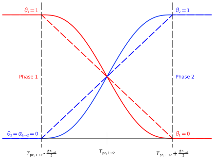
How the phase transition from phase 1 to phase 2 takes place is described by the phase transition function α 1 → 2. By default, COMSOL uses a smoothed step function with a continuous second derivative (Heaviside function). It describes a continuous transition from phase 1 to phase 2 within the transition interval ΔT around the phase transition temperature Tpc. Besides the frequently used Heaviside function, a linear function is also common and available as predefined option.

Figure 4-2 illustrates the functions and the corresponding parameters.

With a user-defined phase transition function, the volume fraction of phase 2 is explicitly specified. For reasonable results, the value range of α 1 → 2 should be between 0 and 1 satisfying θ1 + θ2 = 1 and the function should be differentiable to correctly approximate the latent heat contribution, which is calculated from the derivative of this function by Equation 4-49. A user-defined function can also be used to describe a phase transition where not the complete volume fraction of one phase changes into the other, that is, there is a residual phase.