PML Implementation
PMLs apply a complex coordinate stretching in one, two, or three directions, depending on how the PML domain connects to the physical domain. In each direction, the same form of stretching is used, defined as a function of a dimensionless coordinate ξ, which varies from 0 to 1 over the PML layer. The function returns a new, complex and stretched, coordinate interpreted as relative to the typical wavelength for each simulation frequency. That is, the complex displacement for stretching in a single direction is Δx = λfi(ξ) − Δwξ, where λ is a typical wavelength and Δw is the original width of the PML (as drawn in the geometry). A separate displacement is computed for each stretching direction and summed to make a total displacement.
In the PML nodes, you can choose between predefined polynomial and rational stretching functions, or select your own user-defined functions. The polynomial stretching function is defined as
where p is a curvature parameter, and s is a scaling factor. The rational stretching function is defined as
where p and s are again a curvature parameter and a scaling factor, respectively.
For user-defined stretching, you specify the real and imaginary parts of f(ξ) as separate functions of one or two arguments. The first argument is interpreted as the dimensionless distance ξ and the second — optional — argument as the typical wavelength λ.
For more information about the use of PMLs in acoustics simulations, see Perfectly Matched Layers (PMLs) in the Acoustics Module User’s Guide.
Interpreting PML Parameters
The predefined PML coordinate stretching functions are controlled by three parameters:
The typical wavelength represents the longest wavelength of propagating waves in an infinite medium. It is normally provided by a physics interface. For nondispersive media, it is expected to be inversely proportional to the frequency and serve to make the PML perform similarly for all frequencies.
In eigenfrequency studies, the typical wavelength parameter must not depend on the — unknown — frequency. When the typical wavelength is set to be obtained from a physics interface, it is therefore redefined to be equal to the PML width Δw instead. A user-defined typical wavelength applies as entered, but must not be a function of the frequency. It is often most convenient to draw and mesh the PML as if it had been part of the physical domain. To tune its effective thickness, use the scaling factor.
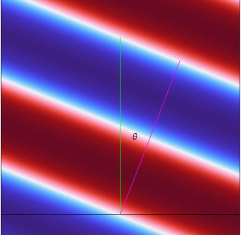
The PML scaling factor multiplies the typical wavelength to produce an effective PML thickness. The absorbing power of the PML is a function of the number of effective wavelengths across the PML in the stretching direction. For example, to retain good absorption for plane waves incident at an angle θ relative to the boundary normal, the PML has to be made thicker by setting the scaling factor to 1/cos(θ); see Figure 5-14 below. This will keep the PML one effective wavelength thick also for oblique incidence.
Figure 5-14: Typical wavelength (magenta) and effective wavelength in the stretching direction (green).
Conversely, if resolving the field inside the PML proves too costly, it is possible to lower the scaling factor below its default value of 1, to make better use of the available mesh elements. Note that this has a price in terms of less efficient absorption.
The PML curvature parameter serves to relocate mesh resolution inside the PML. When there are components present which decay inside the PML much faster than the longest waves, the resolution must be increased in the zone closest to the boundary between PML and physical domain. Increasing the curvature parameter effectively moves available mesh elements toward the inner PML boundary. This is often necessary when the wave field contains a mix of different wavelengths or a mix between propagating and evanescent components.
Choosing a Stretching Type
Which coordinate stretching type is most appropriate depends on the problem at hand. Consider the following when choosing between polynomial and rational stretching:
Polynomial
The polynomial stretching strategy makes a minimum of assumptions about the wave field incident on the PML. Its finite and equal real and imaginary parts mean that propagating and evanescent waves with the same length scale are treated alike. The default scaling factor gives a PML with a maximum attenuation of about 109 dB for normal incidence and provided sufficient mesh resolution.
The polynomial stretching is generally applicable and most appropriate when there is a mix of different wave types in the model and you can afford at least 8 mesh elements across the PML. Also, compared to the rational stretching, it interferes less with the convergence of iterative linear solvers.
Rational
The rational stretching is designed for propagating waves of mixed wavelengths and angles of incidence. The real part of the stretching scales the effective PML thickness to a quarter of a typical wavelength, while the imaginary part — responsible for the attenuation — is stretched out toward infinity. This means that provided sufficient mesh resolution, the PML absorbs any propagating wave perfectly.
User defined
If none of the above stretching types are suitable, you can specify a user-defined stretching using functions that you add to the model as the real and imaginary parts of the stretching function.
In reality, the mesh resolution limits the effectiveness of the rationally stretched PMLs. For a single wavelength at normal incidence, 3 mesh elements across the PML normally give sufficient attenuation and accuracy. If the wave field contains also longer- or shorter-wavelength components, the mesh resolution must be increased. When other wave components are shorter than the supplied typical wavelength, increasing the curvature factor may be useful to make best use of the available resolution.