Port

The boundary condition is used to excite and absorb acoustic waves that enter or leave waveguide structures, like small ducts or channels, in an acoustic model. The thermoviscous port formulation ensures that the nontrivial mode shapes of the acoustic velocity and thermal fields are captured correctly.

A given port condition supports one specific propagating mode. To provide the full acoustic description, combine several port conditions on the same boundary. Typically, only the plane wave mode is propagating in small structures where the thermoviscous representation is necessary. The port condition provides a superior nonreflecting or radiation condition for waveguides compared to a simple impedance condition or a perfectly matched layer (PML) configuration. The same port boundary condition feature should not be applied to several waveguide inlets and outlets. The port condition supports S-parameter (scattering parameter) calculation but it can also be used as a source to just excite a system.

The boundary condition exists for 3D, 2D, and 2D axisymmetric models.


	Only one port should be excited at a time if the purpose is to compute S-parameters. The S-parameters are defined as ta.S11, ta.S21, and so on, and can be used in postprocessing. In other cases, having more than one port exciting the system might be wanted, but the S-parameter variables cannot be correctly computed. So, when several ports are excited, the S-parameter output is turned off. If only two ports are added to the system and a port sweep is performed, the system transfer matrix and system impedance matrices are also computed.

On a given boundary, a combination of ports will define the total acoustic fields (sum of incident and outgoing pressure, temperature, and velocity waves) as

where the summation “i” is over all ports on the given boundary “bnd”, Sij is the scattering parameter, Ain is the amplitude of the incident field and

the phase (at port “j”), and pi, ui, and Ti are the mode shape of the ith port. The mode shape is normalized to have either a unit maximum amplitude (for the pressure pi) or carry unit power (see the normalization option in the Global Port Settings section). For both definitions the scattering parameter Sij defines the amplitude of mode i when a system is exited at port j (with mode j). For the power scaling, |Sij|2 directly gives the power of the given mode. This corresponds to a multimode expansion of the solution on the given boundary. The scattering parameters are automatically calculated when an acoustic model is set up with just one port exciting the system. To get the full scattering matrix The Port Sweep Functionality can be used.

Port Properties

Enter a unique . Only nonnegative integer numbers can be used as as it is used to define the elements of the S-parameter matrix. The numeric port names are also required for the port sweep functionality. The port name is automatically incremented by one every time a port condition is added.

Select a : (the default), , , , or . Depending on the selection, different options appear in the section (see below). Use the for a port with a circular cross section in 3D or 2D axisymmetry and the option in 2D. If the port has a different cross section than either of these, use the option or the port. The option represents a situation where the boundary layers are not included; this is for example for a wave propagating in free space or when slip and adiabatic (or symmetry) conditions are applied to all adjacent boundaries.

Port Mode Settings

Depending on the option selected in the (see above):

•

For , enter user defined expressions for the pn, un, Tn, and the kn (SI unit: rad/m). The mode shape will automatically be scaled before it is used in the port condition. Use the user-defined option to enter a known analytical expression or to use the solution from The Thermoviscous Acoustics, Boundary Mode Interface. The solutions from the boundary mode analysis can be referenced using the withsol() operator.

•

The port options is used for waveguides of arbitrary cross sections. In this case, the shape of the propagating plane-wave mode (0,0) is solved on the port face. The boundary conditions for the mode are taken from the adjacent waveguide boundaries. This automatic detection works for slip, no-slip, adiabatic, isothermal, and symmetry conditions (including the same options when selected in the condition). If all the adjacent wave guide boundaries are slip and adiabatic (or symmetry) then use the option.

For this option, a special solver sequence is automatically generated since the port mode shape (the port variables psi, Psi_th, Psi_v, and vip) should be solved before the domain problem (the main degrees of freedom p, u, T, and Sparam1). If an iterative solver suggestion is to be used, keep the linear solver for the first segregated step and then select the iterative suggestion for the second segregated step. If the port option is selected after a solver has already been generated, then select in the study to get the correct settings.

•

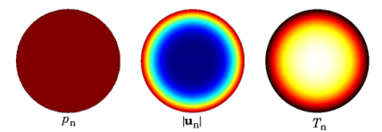
The port option is used for waveguides of circular cross section. The analytical mode is a plane-wave mode (0,0) given by a constant cross section pressure, no-slip condition for the velocity, and isothermal condition for the temperature. An example of the propagating mode shape in a cylindrical waveguide is seen below.

Figure 6-1: Plane wave mode for a circular duct of 1 mm diameter at f = 250 Hz.

Select how the of the cross section is defined, either (the default) or . The latter option can for some geometry configurations increase the numerical precision of the computed mode.

•

The port option only exists in 2D on a boundary. In 2D, the geometry is assumed infinite in the out-of-plane direction and represents a slit. The analytical mode is a plane-wave mode (0,0) given by a constant cross section pressure, no-slip condition for the velocity, and isothermal condition for the temperature.

•

The port option represents a situation where the boundary layers are not included in the mode shape, this is, for example, for a wave propagating in free space or when slip and adiabatic (or symmetry) conditions are applied to all adjacent boundaries.


	The solution for the numeric port is obtained using the generalized low reduced frequency (LRF) approximation commonly used in thermoviscous acoustics. The theory is based on an order of magnitude analysis of the full thermoviscous equations and on the assumption of a plane propagating mode (constant pressure in cross section). The circular and slit options use an analytical solution for the given cross section. The mode shapes based on LRF approximation are valid as long as the wavelength is much larger than the waveguide cross section (λ >> a) and the wavelength is much larger than the boundary layer thickness (λ >> δvisc and λ >> δtherm).

Port Geometry

The settings in this section ensure that the correct port area (including symmetries) is used for computing important quantities like power, volume flow, and transfer matrix elements, associated with the port

Select the as (the default) or .

•

When is selected, symmetry conditions adjacent to the port will automatically be taken into account if the is set to (the default); if set to , enter the area multiplication factor Ascale manually.

•

When is selected, the port will have the area of the selected boundaries, without taking any symmetry conditions into account.

Incident Mode Settings

Activate if the given port is excited by an incident wave of the given mode shape. For the first condition added in a model, the is set to . For subsequent conditions added the excitation is set to per default. If more than one port in a model is excited, the S-parameter calculation is not performed.

When the is set to , then select how to define the incident wave. Select the as (the default) or ( in 2D models)

•

For enter the amplitude Ain (SI unit: Pa) of the incident wave. This is in general defined as the maximum pressure amplitude for a given mode shape.

•

For enter the power Pin (SI unit: W) of the incident mode. In 2D models this will be a (SI unit: W/m).

•

Enter the phase

(SI unit: rad) of the incident wave. This phase contribution is multiplied with the amplitude defined through the above two options. Those inputs can be complex numbers.

Note that when the option is selected at the physics level, the options in the section are deactivated. This is because this option automatically sends in a mode of unit amplitude, sweeping through one port at the time.


	All ports with incident wave excitation turned off have an arrow symbol, added in the Graphics window, that points outward. When incident wave excitation is turned on, the arrow symbol points inward.


	If a waveguide is cut with one or several symmetry planes, care should be taken when setting up the port modes and when postprocessing. For the Circular and Slit options, make sure to only select modes that are actually symmetric according to the symmetry planes.

Constraint Settings

To display this section, click the button (

) and select in the dialog box.

Excluded Edges/Points

To display this section, click the button (

) and select in the dialog box. See Suppressing Constraints on Lower Dimensions for details

The Port Sweep Functionality

The port sweep functionality is used to reconstruct the full scattering matrix Sij by automatically sweeping the port excitation through all the ports included in the model. When the port sweep is activated, the options in the in the port conditions are deactivated and COMSOL controls which port is excited with an incident mode.

The port sweep functionality is activated at the main physics interface level by selecting in the Global Port Settings section. Enter the , the default is PortName. Create a parameter with the same name under . This is the name of the parameter to be used in a parametric sweep; it should represent the integer values (defined when adding the port conditions). Add a parametric sweep study step and run the sweep over the PortName parameter with an integer number of values representing all the ports in the model. Once the model is solved, the full scattering matrix can be evaluated using the defined global variables ta.S11, ta.S21, ta.S12, and so on. The transmission loss (TL) between two given ports is also computed, for example, the variable for the TL loss from port 1 to 2 is given by ta.TL_12.


	Use the Global Matrix Evaluation under Derived Values to evaluate the full scattering matrix ta.S.

If only two ports are added to the thermoviscous model, COMSOL also automatically computes the transfer matrix of the system (variables ta.T11, ta.T12, ta.T21, ta.T22) and the impedance matrix of the system (ta.Z11, ta.Z12, ta.Z21, ta.Z22). These expressions are only true if plane wave modes are used. This is the case in nearly all configurations when working with microacoustic systems. For ports in thermoviscous acoustics, the , , , and options are for plane waves only, that is, the (0,0) mode with varying boundary conditions. Higher-order modes can only be introduced with the option. The transfer matrix representation is often used in electroacoustic modeling.

•

Wax Guard Acoustics: Transfer Matrix Computation. The Application Library path:

•

Transfer Impedance of a Perforate. The Application Library path: