Impulse Response Plot and Receiver Dataset

The impulse response (IR) in a room acoustics simulation can be analyzed by collecting the ray information using the dataset and then postprocess using the plot. Room acoustic metrics like reverberation times, early energy metrics, and speech intelligibility can also be postprocessed using the subfeature. The IR can be determined for sources and boundary data (absorption coefficients, scattering parameters, source directivity, volume attenuation, and so on) given in octave, 1/3 octave, or 1/6 octave bands.

When setting up a Ray Acoustics simulation and preparing it for a room acoustics simulation where the impulse response (IR) is an important output, certain considerations and steps need to be taken. They are as follows:

•

Create parameters under for the band center frequency and the source power, for example, f0 and P0 respectively.

•

Set up interpolation functions for the properties that depend on the frequency. The data can easily be stored in a formatted file and interpolation can be set to . An example of the format for a .txt file that specifies absorption coefficients for some boundaries in a simulation could be (data is invented):

•

Create parameters under for the receiver radius and number of released rays. These two quantities are linked by the expected error in a given time interval Δt of the impulse response, see Ref. 6 for details. With the room volume V, the receiver radius R, and for an expected error of 1 dB, the number of released rays N needed is

The receiver radius can be taken as R = 0.3 m to match the width of a common seat, and a standard time interval is Δt = 0.01 s. For small rooms or car cabins it can be useful to set a receiver radius that represents the actual size of a microphone or slightly larger. The value obtained from this calculation should be rounded up to ensure an integer number of released rays. A higher value can also be chosen and will result in increased resolution.

•

Make sure that either the or the option is selected in the Intensity Computation section. The option requires fewer degrees of freedom and is more robust. If it is selected, the ray intensity (rac.I and rac.logI) cannot be visualized in ray trajectories plots, but both the Sound Pressure Level Calculation on boundaries and the impulse response can be computed.

•

Set up the ray acoustics model with appropriate boundary conditions and sources. Generally, all should be set to , with a default scattering coefficient s = 0.05 for flat surfaces.

•

Create a node and choose as . Select as and enter the threshold P0/N*1e-6. For an omnidirectional source, this expression makes rays disappear once the power they carry has dropped by 60 dB from its initial value.

•

To be able to postprocess the IR, a needs to be used in the study around the study step. The sweep parameter should be the frequency defined in the parameters. To easily create a representing the center frequencies of the bands use the entry method.

•

For the , specified under the study step, only enter 0 and the final simulation time (the final time should be slightly larger than the estimated reverberation time). COMSOL uses small internal steps that accurately account for all reflections. The so-called are used when reconstructing the IR and other data (see below).

Use a (

) or dataset (

), selected from the submenu and the submenu, respectively, to collect the data necessary to visualize the impulse response using an Impulse Response Plot. The plot uses the data from a dataset as input

Select the appropriate ray dataset in the list. Then select the frequency parameters that should be used by the receiver; select one frequency for a single band analysis or all for the broad band analysis. This is the typical behavior if a parametric sweep has been set up, as described in Preparing a Room Acoustics Simulation.

The receiver behaves as a (transparent) sphere with a given radius and located at a center position (the microphone needs to have a certain finite size such that there is a reasonable probability of rays interacting with it). By changing the center position, the receiver can be moved around without the need to run the simulation again.

•

Under , specify the radius of the receiver. From the list, choose to determine the radius using an expression (see below), or choose to enter a value for the radius in the field (SI unit: m). Different theories exist for the appropriate size of the receiver. For room acoustic applications, it is recommended to use a fixed radius from which the number of rays can be derived, as described in Preparing a Room Acoustics Simulation.

where you enter the values for the , N; , V (SI unit: m2); and , dSR (SI unit: m), to determine the radius. See Ref. 19 for details on the expression. This computed receiver size is optimized for modeling of large rooms. However, it will return a different value for each source-receiver pair if there are multiple sources and receivers present in the simulation, and it will not necessarily correspond to the dimensions of a listener.

From the list, choose (the default), , or and enter a directivity expression in the field.

The expression can depend on the ray direction vector components (rac.nix, rac.niy, rac.niz) in order to set up a complex directivity pattern.

Use the default option. The impulse response plot has been tuned to use this option in order to get accurate and fast evaluation of arrival time and ray power.

For the list always use the default interpolation option. The interpolation is not applicable for the impulse response computation and can lead to erroneous results.

Under and , if desired, you can change the default names of the created variables:

The main purpose for the dataset is to be used as input for the Impulse Response Plot. However, the data generated by the dataset can also be exported and used in an external analysis tool or software (ray power and arrival times).

Right-click the dataset and select , then enter the desired data. For example, export the arrival time of the rays t, the frequency of the rays rac.f, the power of the rays rac.Q, the distance traveled by the rays in receiver re1dist, and so forth. The exported data can be stored and sorted in several formats.

When working with phase alignment of loudspeakers, it can be useful to evaluate the arrival time if the first ray. This is easily done in a feature that points to the receiver dataset. Simply evaluate the special variable re1first.

	See also the Receiver 2D and Receiver 3D section in the COMSOL Multiphysics Reference Manual.

In room acoustics applications, the impulse response (IR) of a source-receiver configuration represents one of the most important postprocessing results. To create the plot based on the data collected by the dataset, add an subnode (

) to a 1D Plot Group to create the impulse response plot. After defining the characteristics of the impulse response, click (

) to create the plot. The (

) subnode can be added to perform an analysis of the impulse response to get room acoustic metrics and the energy/level decay curves. The first rendering of the IR plot can take some time. As the data is cached, any subsequent changes to the plot will be fast.

	The Small Concert Hall Acoustics model is a tutorial on how to compute the impulse response using the Ray Acoustics interface. Application Library path: Acoustics_Module/Building_and_Room_Acoustics/ small_concert_hall

In the ray tracing methodology it is, as discussed above, typical to characterize sources and boundaries in frequency bands. This also means that some of the frequency content is lost. This frequency content is reconstructed when determining or reconstructing the IR. For each ray that interacts with the receiver, a small piece of signal with appropriate amplitude, arrival time, phase, and frequency content is added to the IR (the filter bank kernel). The sum of all the contributions reconstruct the full IR.

From the list, choose the appropriate Receiver Dataset. Then from the list choose an interpretation of the frequency: (the default), , or . This selections should coincide with the frequency interpretation used in boundary conditions and sources in the underlying ray acoustics simulation, as described in Preparing a Room Acoustics Simulation. The frequency content and resolution of the impulse response is based on this selection.

Set up the variables that are necessary for reconstructing the impulse response (typically use the defaults). These variables are used to define and add the contribution of each ray, that intersects the receiver dataset, to the impulse response.

From the list, choose a transformation of the data on the x-axis: (the default), for no transformation, to show the time domain signal, or . The latter will perform an FFT of the IR and depict the power spectra as function of frequency.

The following advanced settings are available to control some aspects of the IR reconstruction as well as the underlying filter kernel used.

The next two options are legacy options (to achieve behavior for COMSOL Multiphysics releases older than version 5.6).

•

Select to remove the signal (force it to zero) prior to the arrival of the first ray. Using this option will alter the energy content of the early energy component of the IR.

•

Select to use the legacy method for reconstructing the IR. The fully randomized phase method (see Ref. 20) can lead to unwanted cancellations of the direct sound and early energy contributions.

The following options control the filter kernel used to reconstruct the impulse response. Advanced options allow to modify the kernel, enter a user-defined analytical kernel, or a user-defined kernel based on an interpolation function. The default is to use a Brick-wall with Kaiser window filter kernel (see Ref. 21).

•

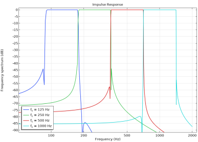
Select to show and inspect the filter bank in the window, click (

) to create the plot. To switch between time domain and frequency domain representation change the option in the section.

•

Select the to use (the default) or . When is selected enter the expression for the filter kernel hfc[t]. Use and set up parameters in the table (as you would use variables). The parameter fc is reserved for the (exact) band center frequency; fr is reserved for the ray frequency (this is typically the nominal band center frequency selected in the study); fs is reserved for the sampling frequency; t is for time; and Np is the padding length. Note that per default the option sets up the brick-wall with Kaiser window filter kernel for octaves.

•

If the default is selected, you can control the ripple factor δ (the default is 0.05). The effect on the filter can be seen using the option.

You can also make change in the section or add and format a legend in the section.

	See also the Impulse Response section tn the COMSOL Multiphysics Reference Manual.

For further analysis of the impulse response, add the (

) subnode to the plot. Once selections have been made, click (

) to create the plot.

Select the as (the default) or . For the option select the , either an individual band or . For , all the level or energy decay curves are plotted.

Select the as (the default), , or , to define the type of graphical analysis of the impulse response to be plotted in the window.

Select the room acoustic metrics to be included in the results table, per default all objective quality metrics are selected. The default name of the table is . The table displays the results in columns with the band center frequency fc in the first column. The results table can also be located under the node. A plot of the results located in the table can be created using the plot.

	The speech transmission index (STI) metric is defined as a single value that combines information from 14 modulation transfer function bands and 7 octave bands. To get the value specified by the standard solve the model for octaves from 125 Hz to 8 kHz. When evaluating use the Band type set to the default Broadband option.

The energy response depicted as a reflectogram or echogram can be plotted using a Ray (Plot) and depict the expression re1dist*rac.Q/re1vol. This will give the intensity received by the “microphone” for each ray.