In COMSOL Multiphysics you can model contact between a group of boundaries in 2D or 3D. There are two classes of algorithms available: the penalty method and the augmented Lagrangian method.

A prerequisite for setting up the mechanical contact problem is to define the contact search between the source boundary and the destination boundary. The purpose of the search is to detect points on the contacting boundaries that are in contact or may come in contact, and also to map quantities between such points. This part of the contact problem is defined in the Contact Pair that sets up relevant variables and operators to map quantities between the selected source and destination boundaries. In COMSOL Multiphysics, the contact search is made using a ray-tracing strategy as depicted inFigure 3-34. For mechanical contact, most variables and equations are formulated on the destination boundary. Hence, the typical mapping of interest here is from the source boundary to the destination boundary, however, it is possible to map quantities in the opposite direction as well.

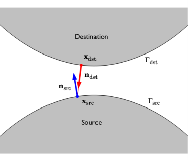
For each point xdst in the spatial frame on the destination boundary Γdst, the closest point xsrc in the spatial frame on the source boundary Γsrc in the direction of the destination spatial normal ndst is sought. Such a mapping can be described through and operator map(E, x), where E is some generic quantity or expression, and x is the point to which E is mapped. Using this mapping operator, the coordinates of the mapped point on Γsrc is

where x is the spatial coordinates that parameterize Γsrc. For brevity, the second argument of the mapping operator is omitted in the following and it should be understood that the mapping occurs to a point xdst on Γdst if nothing else is specified.

An important quantity for contact mechanics is the gap function ggeom(x) defined as the geometric distance between the source and the destination boundary. Note that ggeom(x) is not necessarily the closest distance between the two boundaries. Using the mapping operator, the gap distance at xdst is defined as

With the above definitions, a positive gap infers that there is a geometrical separation between the points, while a negative gap that there is an overclosure. Apart from the mapping operator, the Contact Pair also defines a dedicated variable for the gap function with the name geomgap_dst_<pair_tag>.

For the mechanical contact problem, it is additionally possible to define a physical offset from the geometric source and destination boundary. This means that the physical gap function gn(x) and geometrical gap function do not necessarily coincide. The physical gap distance including offsets at xdst is defined as

where doffset,s and doffset,d is the offset from the source and destination boundary, respectively. Each offset variable can vary along the geometry, and may also vary in time (or by the parameter value when using the continuation solver). The correction of the source side offset is necessary since the normal of xsrc, nsrc=map(n), is not necessarily pointing towards xdst as illustrated in Figure 3-34. When the geometric surfaces are in contact, the normals will be exactly opposite.

In some cases, the discretization of the geometry, especially at curved boundaries, will give small irregularities in the gap function. You can then choose to adjust the physical gap by removing the geometric gap computed in the initial configuration, ginit, smaller than the tolerance Δgap. In this case, the physical gap function at xdst is

For problems including friction or adhesion, it is also necessary to know the tangential movement, or slip, between the source and destination boundary. The rate of the relative slip vector gt between the two boundaries at xdst is defined as

where X is the material coordinates, and F is the deformation gradient that contains information about the local rotation and stretch. Both quantities are mapped from the source to the destination boundary. Constitutive models for the mechanical problem are typically formulated on an incremental form. COMSOL Multiphysics applies a backward Euler approximation to Equation 3-162 so that the incremental slip at xdst is

where Xsrc,old is the mapped material coordinates at the previous increment.

The contact constraint in the normal direction to the contacting boundaries can be represented by the non-penetration condition. On the destination boundary Γdst, the normal contact condition can be written as a weak equation (the contribution of normal contact to the virtual work)

where Tn is the contact pressure, assumed positive in compression. To complete the contact condition, Equation 3-163 is subjected to the Kuhn–Tucker conditions

where the first inequality represents the nonpenetration condition. Equation 3-163 and Equation 3-164 together represents a unilateral constraint that require special techniques to implement. Several different techniques for doing so are available in COMSOL Multiphysics, which can be divided into two main classes: the penalty method and the augmented Lagrangian method.

For the penalty method, the contact pressure in Equation 3-163 is represented using a penalization of the physical gap so that

where pn is the penalty factor, and p0 is the pressure at zero gap. This leads to an approximative solution of the non-penetration condition. The penalty method as defined by Equation 3-165 is conceptually based on the insertion of a nonlinear spring between the contacting points. The penalty factor can be interpreted as the stiffness of that spring. A high value of the stiffness enforces the contact conditions more strictly, but if it is too high, it makes the problem ill-conditioned and unstable.

The pressure at zero gap, p0, can be used to reduce the overclosure between the contacting boundaries if an estimate to the contact pressure is known. In the default case, when p0 = 0, there must always be some overclosure in order for a contact pressure to develop.

In addition to Equation 3-165, COMSOL Multiphysics also provides an alternative penalization based on a viscous formulation intended for transient simulations, referred to as the Penalty, dynamic method. This formulation is based on the additional persistency condition

where gn,old is the physical gap distance at the previous increment, and <> is the positive parts operator. With the definition in Equation 3-166, Tn is only non-zero if the physical gap is negative during the entire increment, which is important for energy conservation during the initial contact event. However, there will always be some initial penetration before the gap rate is penalized. Hence the observed overclosure will be dependent on the size of the increment when two points come into contact. Note that this definition of the contact pressure implies that pressure contact is dissipative.

It is possible to use the definitions of Tn in Equation 3-165 and Equation 3-166 simultaneously. In such a case, they are additive and conceptually represent a parallel coupling of a spring and a dashpot.

The augmented Lagrangian method can be seen as a compromise between using the penalty method and enforcing the non-penetration condition using weak constraints and Lagrange multipliers. The augmented Lagrangian formulation for normal contact in COMSOL Multiphysics is based on an integral formulation that in a weak sense enforces the non-penetration condition exactly over the contacting boundaries. It is based on the following augmentation of Equation 3-163

where Tnp is the penalized (or augmented) contact pressure, and Tn is a Lagrange multiplier that can be identified as a contact pressure. The Lagrange multiplier representation of the contact pressure is defined as the dependent variable of the contact problem and is typically discretized using Lagrange shape functions. There are two methods for solving the above coupled system of equations, and this choice affects the definition of Tnp.

The first solution method is referred to as a Segregated method and corresponds to the so-called Uzawa algorithm. Here, the system of equations is decoupled, and the displacement field u and the Lagrange multiplier Tn are solved in a segregated way. This leads to two levels of iterations in the solver, where Tn is held constant when solving for u, and vice versa when updating Tn. For this solution method, the penalized contact pressure Tnp is defined with a smooth transition to stabilize the problem when transitioning between contact states. The definition for Tnp for outer iteration j+1 is defined by

The segregated method can then for increment n+1 schematically be described as

The appropriate solver sequence is automatically set up by COMSOL Multiphysics for the Segregated solution method when adding a new solver, or resetting to the default solver.

The alternative is to use a Fully Coupled solution method, which, as the name implies, amounts to solving the coupled system in Equation 3-167 for the two dependent variables u and Tn (and any other variables included in the multiphysics model). When using this method, the penalized contact pressure is defined by

The Fully Coupled method can be convenient as it enforces the non-penetration condition exactly over the contacting boundaries, while it puts no restriction on how to set up the solver sequence. This flexibility can be especially advantageous when working with multiphysics problems, compared to the segregated approach. However, one should be aware that the method comes with some of the drawbacks of a pure Lagrange multiplier approach, albeit to a lesser extent. One drawback is that the solution typically is a saddle point, and convergence can be sensitive to how Newton iterations are made when solving the nonlinear problem.

In the limit, the Segregated and the Fully Coupled solution methods converge to the same solution, but they can have different convergence properties.

In addition to the standard augmented Lagrangian method outlined above, an Augmented Lagrangian, dynamic method is available for transient simulations. As discussed for the penalty method, this formulation is based on the addition of the persistency condition. A segregated solution method is recommended for this method, and the main difference compared to the standard method lies in the definition of the penalized contact pressure. Both the non-penetration and persistency conditions are enforced by penalizing the rate of the physical gap distance so that

where gn,old is the physical gap distance at the previous increment, and <> is the positive parts operator. The same segregated solution strategy as described above is applied also when the dynamic method is used.

The Penalty, dynamic and Augmented Lagrange, dynamic methods are based on a viscous type formulation, and dissipate energy when the contact is active. The accumulated dissipated energy Wcntv can be computed by solving a distributed ODE on the destination boundary:

The tangential behavior of a contact interface, due to friction, can be divided into two states, the stick state and the slip state. The stick state is simply defined by the constraint that there can be no tangential movement between the two contacting boundaries. When the contact enters the slip state, the tangential condition enforces the direction of the relative tangential motion between points xdst and xsrc on the respective side of the interface. On the destination boundary Γdst, the tangential contact condition can be written as a weak equation (the contribution of tangential contact to the virtual work)

where Tt is the friction force. The stick and slip conditions are then enforced by the constitutive model used to define Tt.

where Fslip is the slip function (analogue to the yield function in plasticity theory), and λ is friction multiplier. The critical friction force Tt,crit determines when slip occurs, and is defined as

where Tcohe is the cohesion, and Tt,max defines the maximum friction force that is admissible. The friction coefficient μ can either be defined as an arbitrary constant expression or through an exponential decay model in time-dependent studies. The latter model is defined as

where μstat is the static friction coefficient, μdyn is the dynamic friction coefficient, vs is the slip velocity, and αdcf is a decay coefficient.

It is possible to also define the critical friction force through an arbitrary expression. In principle, Tt,crit, or any variable described above, may be defined as a function of any other variable or field. However, the implementation described in the following is only valid as long as it does not dependent on Tt. In other words, the implementation of the friction constitutive model does not allow for hardening behavior of the friction force.

In COMSOL Multiphysics, implementation of Equation 3-170 is made using a backward Euler integration. Together with a penalty regularization, this results in the following set of algebraic equations to solve at increment n+1:

where Tt,n is the friction force at the previous increment. The set of algebraic equations is solved for unknowns Tt,n+1 and λ by introducing a trial state and a return mapping. In doing so, it is assumed that Tt,crit, n+1 is independent of Tt, n+1, which leads to an explicit set of equations for finding Tt, n+1. The trial state is first computed as

The weak contribution added for tangential contact when using the penalty method follows from Equation 3-169, and is given by

where Ttp is the penalized (or augmented) friction, and Tt is a Lagrange multiplier that can be identified as a traction. The Lagrange multiplier representation of the tangential traction is defined as the dependent variable of the contact problem and is typically discretized using Lagrange shape functions. There are two methods for solving the above coupled system of equations, Segregated and Fully coupled, as selected in the parent Contact node.

As for the penalty method, Equation 3-170 is implemented using backward Euler integration of the evolution equations, and a trial state and return mapping to solve the nonlinear algebraic equations.

When the Segregated solution method is selected in the parent Contact node, the trial state for outer iteration j+1 is computed as

This scheme then fits in to the algorithmic format described for normal contact where the displacement field u and the Lagrange multipliers associated with contact are solved in a segregated way. Including friction, this algorithm is schematically described as

The segregated algorithm is also used when friction is used together with the Augmented Lagrangian, dynamic formulation.

When the Fully coupled solution method is selected in the parent Contact node, the trial friction force for iteration i+1 is computed as

The weak contribution added for tangential contact when using the Fully coupled solution method follows from Equation 3-171, and is

In the Slip Velocity subnode to Contact, it is assumed the tangential contact is in a slip state when in contact, and that the relative motion between the source and destination boundaries is known beforehand. That is

where vslip is the prescribed velocity on the destination boundary relative to the source boundary. Given that the rate of the slip is known, the constitutive model for friction in Equation 3-170 is simplified, and it follows that

since the slip velocity and friction force are co-linear. The weak contribution added for tangential contact by the slip velocity follows from Equation 3-169 and is

Friction is a dissipative process and the accumulated dissipated energy Wfric can be computed by solving a distributed ODE on the destination boundary:

You can model a situation where two boundaries stick together once they get into contact by adding an Adhesion subnode to Contact. Adhesion can only be modeled when the penalty contact method is used. The adhesion formulation can be viewed as if a thin elastic layer is placed between the source and destination boundaries when adhesion is activated.

Using the effective gap distance gn and the slip Δgt, the adhesion formulation defines an incremental displacement jump vector u in the local boundary system as

where Tb-T contains the transform from the global system to the boundary system. In the above expression, the Macaulay brackets indicate the positive parts operator such that

Using the displacement jump vector, the adhesive stress vector f is defined as

where k is the adhesive stiffness. For negative values of gn, the normal component of f is zero, and the contact condition is resolved by the penalty contact formulation. Notice that a different sign convention is used for the normal stress in the adhesion and contact contributions, where Tn is positive in compression.

The adhesive stiffness k can be defined using three different options: From contact penalty factor, User defined, and Use material data. For the first option, the normal stiffness is set equal to the contact pressure penalty factor pn. The two tangential stiffness components are then assumed to be related to the normal stiffness, so that the stiffness vector equals

where nτ is a coefficient with the default value 0.17. This coefficient can either be input explicitly, or be computed from a Poisson’s ratio. A plane strain assumption is used for this conversion, giving

For the Use material data option, k is calculated from the elastic constants of a fictive layer with a thickness equal to ds.

When adhesion is active, it is possible to break the bond between the source and destination boundaries by adding a Decohesion subnode to Contact. Decohesion modifies the stress vector f defined by Adhesion, but does not explicitly add any new contribution to the to the virtual work on the destination boundary. It thus requires an active Adhesion node.

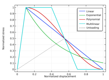
where d is the damage variable. During crack opening (or shearing), the damage variable grows, resulting in a softening behavior of the interface until it eventually breaks when d = 1, see Figure 3-36. If the interface is unloaded, the material follows the linear secant stiffness as defined by the current state of damage. No permanent deformations remain at complete unloading.

The Decohesion subnode implements the second term on the right-hand side of Equation 3-172, while the first term is implemented in Adhesion. Notice that in the normal direction, damage only applies to separation of the boundaries, hence the normal contact is unaffected by decohesion.

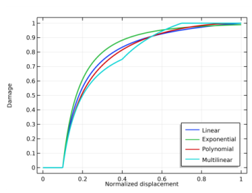
In the displacement-based damage models, the damage variable d is defined using a damage evolution function written in terms of a displacement quantity. Since, in general, the fracture is a combination of mode I and mode II fracture, the model introduces a mixed mode displacement um as the norm of the displacement jump vector.

To keep track of the current state of damage, the maximum value of um over the loading history is defined as

where is and internal degree of freedom that takes the value of um,max at the previous converged solution. The damage variable is then defined as a function of um,max of the form

where F-1 is called the damage evolution function and u0m defines the onset of damage. Conceptually, the damage evolution function is the inverse of the softening branch of the traction separation law F. Four different definitions of F-1 are available in the Traction separation law list. These damage evolution functions are summarized in Figure 3-35, and the resulting traction separations laws in Figure 3-36.

The Linear option specifies a damage evolution function that gives a bilinear traction separation law as seen in Figure 3-36. It is defined as

where u0m and ufm define the mixed mode initiation of damage and point of complete fracture, respectively. For the initiation of damage, a linear mixed mode criterion gives

where uI and uII are the mode I and mode II displacements, respectively. These are obtained from the displacement jump vector u. The constants u0t and u0s are calculated as

where σt is the tensile strength and σs is the shear strength of the adhesive layer. The normal stiffness kn and the equivalent tangential stiffness kt are obtained from the adhesive stiffness vector k. The mixed mode failure displacement ufm depends on the selected Mixed mode criterion. The Power Law criterion is defined as

and the Benzeggagh-Kenane criterion is defined as

where Gct, Gcs and Gcm are the tensile, shear, and total energy release rates, respectively. The exponent α is called the mode mixity exponent. From these relations, the mixed mode failure displacement can be calculated. For the power law criterion, the expression is

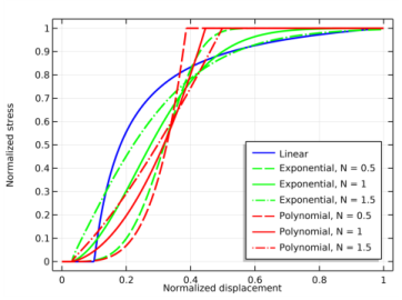
The Exponential option specifies a damage evolution function that gives a traction separation law which is linear up to the interface strength, and thereafter softens with an exponential curve that reaches zero asymptotically as seen in Figure 3-36.

The mixed mode damage initiation displacement u0m is defined by Equation 3-173 and Equation 3-174. The mixed mode failure displacement ufm is for the power law again given by

The Polynomial option specifies a damage evolution function that gives a traction separation law that is linear up to the interface strength. and thereafter softens with a cubic polynomial curve as seen in Figure 3-36.

The mixed mode damage initiation displacement u0m is defined by Equation 3-173 and Equation 3-174, and the mixed mode failure displacement ufm by Equation 3-175 or Equation 3-176.

The Multilinear option specifies a damage evolution function that gives a traction separation law that is linear up to the interface strength. Thereafter a region of constant stress is introduced before the interface softens linearly as seen in Figure 3-36.

The mixed mode damage initiation displacement u0m is defined by Equation 3-173 and Equation 3-174. The new constant upm defines the end of the region of constant stress and requires the introduction of the shape factor λ. The shape factor defines the ratio between the constant stress part of Gct and the total “inelastic” part of Gct:

Note that the shape factor is similarly defined for shear and is assumed to be equal for both components. Setting λ = 0 corresponds to the linear separation law. Using the above expression, the stress plateau displacement upi for the respective component can be expressed as

and the failure displacement ufi as

where index i indicates either tension or shear. For the multilinear option, the mixed mode criterion is always linear (α = 1). Hence the mixed mode stress plateau displacement and failure displacements are given as

The energy-based damage models provide an alternative formulation that relates the growth of damage to the dissipated mechanical energy of the interface. The formulation is based on the work presented in Ref. 4 and Ref. 5. The derivation starts from a stored energy function

From ψ(u, d), the stress vector f and damage energy release rate Ydm are obtained as

To keep track of the current state of damage, the maximum value of Yd over the loading history is defined as

where is and internal degree of freedom that takes the value of Ydm,max at the previous converged solution. The energy dissipated during the decohesion process is

where Gcm is the critical energy release rate in the sense of fracture mechanics. The overall behavior of the cohesive zone model is then summarized by

where Yd0m defines the damage threshold and F is a monotonically increasing function of the damage variable. From the above, an expression for the damage variable is obtained as

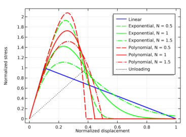
Three different definitions of F-1 are available under the Traction separation law list for the energy-based damage model. These damage evolution functions are summarized in Figure 3-37, and the resulting traction separations laws in Figure 3-38.

The Linear option specifies a damage evolution function that gives a bilinear traction separation law as seen in Figure 3-38.

For the linear law, the equation constant Ydfm = Gcm. The Exponential option specifies a more general damage evolution function of the following form

where N is a smoothening parameter with a default value equal to 1. The effect of N on the traction separation curve can be seen in Figure 3-38. For the exponential law, Ydfm is defined as

where Γ() is the gamma function. A similar damage evolution function is obtained by the Polynomial option. It gives a generalized version of the traction separation law proposed in Ref. 5 of the form

Left to determine are the two variables Yd0m and Gcm. Their definitions require the introduction of a few new concepts related to the mixed mode loading. First, a mixed mode ratio is introduced

where uI and uII are the mode I and mode II displacements, respectively. These are obtained from the displacement jump vector u. The energy release rates of the respective modes are then given by

where G0t and G0s define the damage threshold in tension and shear, respectively. The corresponding criterion for the fracture toughness is

where Gct and Gcs are the critical energy release rates for tension and shear, respectively. The variables α0 and αc are called mode mixity exponents. Using these mode mixture rules results in

Due to the release of energy during decohesion and the softening behavior of the damage models, models may suffer from unwanted mesh dependency. The CZM can suffer from instability leading to nonconverging solutions, or bifurcation causing different solutions for different meshes. Such deficiencies may be alleviated by introducing some additional form of regularization. Under the Regularization list, it is possible to add the Delayed damage regularization. This option adds a viscous delay to the damage growth, and is available with time-dependent studies. The formulation introduces a viscous damage variable dv, and redefines Equation 3-172 so that

where d is the damage variable obtained from any of the available CZM, and τ is the characteristic time that defines the delay of the decohesion. If the viscous damage is used to stabilize a rate-independent decohesion problem, the value of τ must be chosen with care. As a rule of thumb, τ should at least be one or two orders of magnitude smaller than the expected time step. Too large values of τ can introduce significant amounts of extra fracture energy to the model, and the actual energy dissipated due to damage can exceed the defined critical energy release rates by orders of magnitude.

The current value of the viscous damage variable is obtained from numerical integration of Equation 3-177, such that

where Δt is the current time step taken by the time-dependent solver. The value of the viscous damage at the previously converged step is stored as an internal degree of freedom.

where the required values at the previously converged step n are stored as internal degrees of freedom.

By adding a Wear subnode to a Contact node, it is possible to model adhesive or abrasive wear of the material when the contacting boundaries are sliding along each other. Since wear involves solving evolution equations, the Wear node only adds a contribution for time-dependent studies.

The removal of material during the wear process can be modeled with two fundamentally different techniques. The most general technique is to model the removal using the deformed geometry concept. With this approach, the material frame X of the domains adjacent to the contacting boundaries is updated according to the computed wear depth hwear. This means that there is an actual removal of material during the simulation which affects, for example, the contact search, mapping and conditions. When selecting the Deformed geometry formulation, the wear feature adds a (hidden) Deforming Domain feature that controls the material frame through an adaptive mesh smoothing. The removal of material is made through a (hidden) Prescribed Normal Mesh Displacement boundary condition controlled by hwear on the selected contact boundaries. By adding the deformed geometry, an extra dependent variable is added, the material mesh displacement material.disp. This adds a set of extra degrees of freedom to the model that needs to be solved for.

Alternatively, the removal of material can be modeled using an offset-based approach. This formulation offers a simplified approach that is computationally less expensive, but mainly suitable when the amount of worn-off material is small. When selecting the Offset-based formulation, hwear is subtracted from the offset variables doffset,s and doffset,d in Equation 3-161. Hence, the material is considered removed only in the definition of the physical gap, while the contact search and mapping are unaffected. The latter follows from the fact that the actual coordinates and normals of the contacting boundaries essentially remain constant with respect to the wear; they, however, can change due to the deformation induced by the wear and changing contact conditions.

where the rate of the wear depth is given by some source term f that is typically a function of the slip velocity vslip, the contact pressure Tn, and the temperature T. The surface and material properties also play an important role, and are represented by the generic quantity θ in the above equation.

In COMSOL Multiphysics, the wear depth can be computed using a Generalized Archard law for which the wear rate is

Here kwear is a dimensionless wear constant and the exponent n controls the dependence of the wear rate on the contact pressure. The reference contact pressure, Tn,ref, can be chosen arbitrarily, and is used only to obtain consistent units. The classical Archard wear equation is retrieved from Equation 3-178 by setting n = 1 and Tn,ref = 1 Pa. In addition, it is also possible to enter an arbitrary expression for the source term f that defines the wear rate.

It is possible to account for wear on both the source and destination boundaries. However, it is generally more accurate to model wear on the destination side. This follows from the fact that most relevant quantities, such as Tn and vslip, are defined only on the destination boundary in the Contact node and by, for example, the Friction node. Hence, when modeling wear on the source boundary, these quantities are mapped from the destination to the source. For example, when applied to the source side, Equation 3-178 actually reads

The definition of the wear rate thus includes multiple mappings form source to destination, and form destination to source. As described in Contact Search and Kinematics, these mappings are not necessarily one-to-one, which can lead to accumulating errors. The offset-based wear formulation can be especially sensitive to such errors.